What is Geospatial Data

Geospatial data, linked to specific geographic coordinates on the surface of the Earth, forms the basis of how organizations understand, visualize, and take action regarding spatial relationships. Whether it is about monitoring supply chains spanning continents or about finding the best retail locations, geospatial data enables decisions that once could not be made with accuracy.

This article introduces the two main geospatial data models, compares them, presents real-world use cases, outlines the challenges practitioners face, describes how to implement a geospatial data pipeline, and offers best practices for working with spatial data.

Summary of key geospatial data concepts

Concept	Description
Geospatial data	Geospatial data is any data that links a specific location on Earth to a set of attributes. It is typically represented by a combination of coordinates and the feature values associated with them.
Vector and raster data	Geospatial data comes in two forms. Vector data uses points, lines, and polygons to represent discrete features, whereas raster data uses a grid of cells, or pixels, each holding a value.
GIS applications	Geospatial data supports applications in urban planning, logistics and supply chain, environmental monitoring, business intelligence for retail, and similar domains.
Challenges in geospatial data integration	Typical challenges include coordinate reference system mismatches, data volume, data silos, and a lack of frameworks that can integrate geospatial data. The frameworks that do exist carry a steep learning curve.
Best practices	Automated coordinate and geometry validation, a unified coordinate reference system, dynamic schema mapping, and spatial autocorrelation testing are among the best practices to consider when working with geospatial data.

Understanding geospatial data

Real-world spatial phenomena are represented in either vector or raster data models. Each model has its own strengths and weaknesses, and they encode real-world spatial phenomena in fundamentally different ways.

The vector data model

This model represents discrete geographic features by points, lines, and polygons. Each feature is linked to its attributes based on a unique identification number. Vector data models can be structured as either spaghetti or topological models. The diagram below provides a detailed overview of the vector data model.

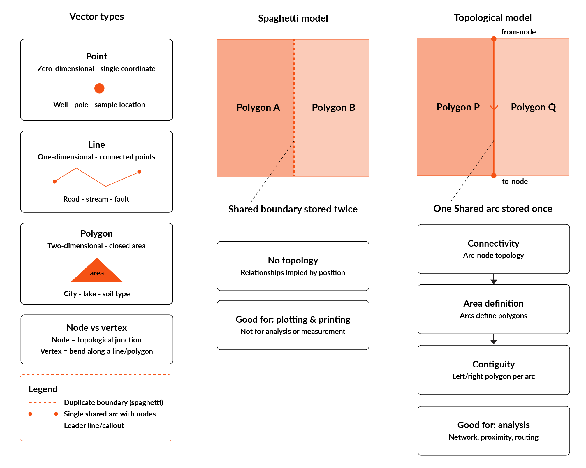
In the spaghetti model, each polygon’s boundary is stored independently, so the shared edge between two neighboring polygons is duplicated. This means there’s no explicit topology and the relationships between features (like adjacency) are only implied by their spatial position. This approach is good for simple plotting and printing, but not for analysis or measurement, since there’s redundancy and no relational structure.

In the topological model, the shared boundary is stored only once. This structure builds up through several layers, such as connectivity, area definition, and contiguity.  Since relationships are explicitly encoded, this model is well-suited for analysis tasks like network analysis, proximity, and routing.

The raster data model

Unlike the vector data model, the raster data model divides geographic space into a regular grid of equal-sized cells named pixels. Each pixel is assigned a single value that might represent elevation, temperature, or population density. The raster data model is more appropriate for representing continuous phenomena and for images obtained by satellites. The spatial resolution of a raster tells us how much area each pixel represents in the real world.

The raster data model has three main categories of data values, each with specific data formats, as shown in the table below.

Value type	Data format	Examples	Typical use
Continuous	Floating-point or integer; any value within a range	Elevation, temperature, precipitation, and slope	Terrain analysis, climate modeling, and hydrological flow
Classified	Integer index referencing a lookup table of class labels	Land cover (e.g., 1=grassland, 2=agricultural, 3=urban)	Land-use mapping, soil classification, and geology
Imagery	Per-band integer (0–255 or 0–65535); one raster layer per spectral band	Landsat bands (red, green, blue, NIR, SWIR)	Change detection, NDVI, land-cover classification, and visual mapping

As for the format, the common vector data formats are as follows:

• Shapefile
• GeoJSON
• GeoPackage 
• File Geodatabase
• KML/KMZ
• PostGIS

Common raster formats include: 

• GeoTIFF
• Cloud-Optimized GeoTIFF
• NetCDF
• HDF5
• JPEG2000
• MrSID

Vector vs. raster 

Choosing between vector and raster data is an important step in a geospatial project because it affects storage, analysis, processing, visualization, and pipeline complexity. However, it is not the only important decision, as the coordinate reference system, scale, and data quality also affect the final result. 

The problem the organization is trying to solve usually determines which model should be used. Vector is more suitable for discrete objects, while raster is more suitable for continuous phenomena. A simple rule is to ask whether the feature has a clear boundary. If yes, vector is usually used; if the values change gradually across space, raster is more appropriate.

Making Spatial Computing Real, Live, and Actionable

Learn MoreLearn More

Connect field workers to an organization’s entire data ecosystem

Visualize, update, and interact with digital twins in real time

Build spatial data pipelines and workflows using a no-code user interface

Use cases of geospatial data 

Here are some classical use cases where geospatial data is critical:

• Urban planning: This is perhaps the most traditional domain for applied geospatial analysis. A practical example is transit-oriented development analysis. City authorities can overlay parcel data with buffer zones around proposed transit stops to identify parcels that fall within a walkable distance. 
• Logistics and supply chain management: Every route, warehouse placement, and last-mile delivery challenge has a spatial dimension. Route optimization engines like those used by DHL, UPS, and Amazon Logistics ingest road network vector data (with attributes such as speed limits, turn restrictions, road class, and time-of-day congestion weights) and solve vehicle routing problems across thousands of delivery stops. 
• Environmental monitoring: Environmental phenomena such as deforestation, coastal erosion, and wildfire spread are examples in which geospatial data, especially satellite imagery, is necessary due to the scale and speed of these events.
• Business intelligence for retail: Geospatial data is essential for decision-making in the retail industry, as it helps retailers determine where to open new stores to serve customers better and respond to competitors. Many geospatial datasets, such as population density, income, age distribution, and customer distribution, are used to find the optimal location. Another use case is competitor proximity analysis to identify locations with market saturation and those with underserved demand.

Challenges in dealing with geospatial data

Geospatial data is complex and not easy to handle. Some of the key challenges while dealing with geospatial data are explained below. 

Issues with the coordinate reference system: CRS mismatches are among the most common and most consequential errors in geospatial workflows. When two layers are rendered in different CRSs without reprojection, features appear displaced, sometimes by hundreds of meters or more. 

Data volume: Traditional desktop GIS tools were not designed for this scale. Processing a global raster dataset in a single-threaded GIS application can take hours or days. Organizations increasingly rely on distributed processing frameworks (e.g., Apache Spark with the Sedona spatial extension or Google Earth Engine’s cloud-based raster processing) and cloud-native data formats (Cloud-Optimized GeoTIFF, Zarr) to handle data at scale.

Data silos and integration challenges: In most organizations, geospatial data is divided up and kept in separate silos, each of which may use different coordinate reference systems (CRSs), feature naming conventions, precision standards, and update schedules. There is a major engineering problem involved in integrating these diverse sources into a single spatial data warehouse.

Data conversion challenges: Geospatial data is frequently obtained from a variety of suppliers and partners in formats including Shapefile, GeoJSON, KML, GeoPackage, File Geodatabase, CAD DXF, and CSV. Each of these formats has its own way of encoding geometry, restrictions on attribute data types, and specific metadata conventions. When converting between formats, several risks are involved, such as attribute field names being truncated, data types being coerced, geometry precision being changed, and CRS metadata being lost or misinterpreted. As a result, it is necessary to have a thorough data conversion pipeline to maintain the accuracy of the geospatial analysis.

Lack of frameworks and the steep learning curve associated with them: One of the biggest barriers to using geospatial data is the lack of a single, easy-to-use framework. The geospatial ecosystem is currently fragmented across many libraries, data formats, and tools, with inconsistent APIs and limited interoperability. This makes it extremely difficult to work with geospatial data, as users must navigate GDAL, Shapely, Fiona, GeoPandas, PostGIS, QGIS, and SDKs. Each format has its own CRS, geometry data structure, and documentation quality. This fragmentation creates a steep learning curve that gatekeeps geospatial work behind a small pool of GIS specialists and slows its adoption. 

The framework issue above is precisely the gap that low-code integration platforms are designed to close. FME, in particular, abstracts the underlying libraries, formats, and coordinate systems behind a visual, drag-and-drop workspace, so engineers can assemble functional geospatial workflows without writing code and become productive in hours rather than weeks. By lowering the technical barrier to entry, such platforms widen access to geospatial work beyond the small pool of specialists and shorten the learning curve described above.

Implementing a geospatial pipeline

The next section builds a simple geospatial pipeline in FME Workbench, the visual workflow-authoring application included with FME Form.

Here, you will build a pipeline that takes raw public data, cleans and validates it, brings it onto a common coordinate reference system, and produces a ready-to-use deliverable, demonstrating the full ingest-to-output sequence that most geospatial integration tasks follow.

The pipeline ingests public OpenStreetMap data for a target city, applies quality filtering and geometry validation, reprojects the data to a standard coordinate reference system, and writes the output to a KML file for use in Google Earth or downstream web mapping applications.

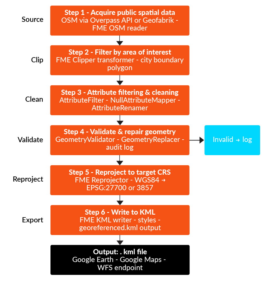
Let’s learn how we can build this step by step.

Step 1: Acquire public spatial data

Source public building-footprint and road-network data for the target city from OpenStreetMap, either through the Overpass API or as a prepackaged extract from Geofabrik; for a city such as London or Nairobi, the OSM extract may arrive as a compressed .osm.pbf. In FME, add an OpenStreetMap (OSM) reader and configure it to read the desired feature types (for example, buildings and highways). FME parses the OSM tags and produces a separate feature stream for each type.

Step 2: Filter by area of interest

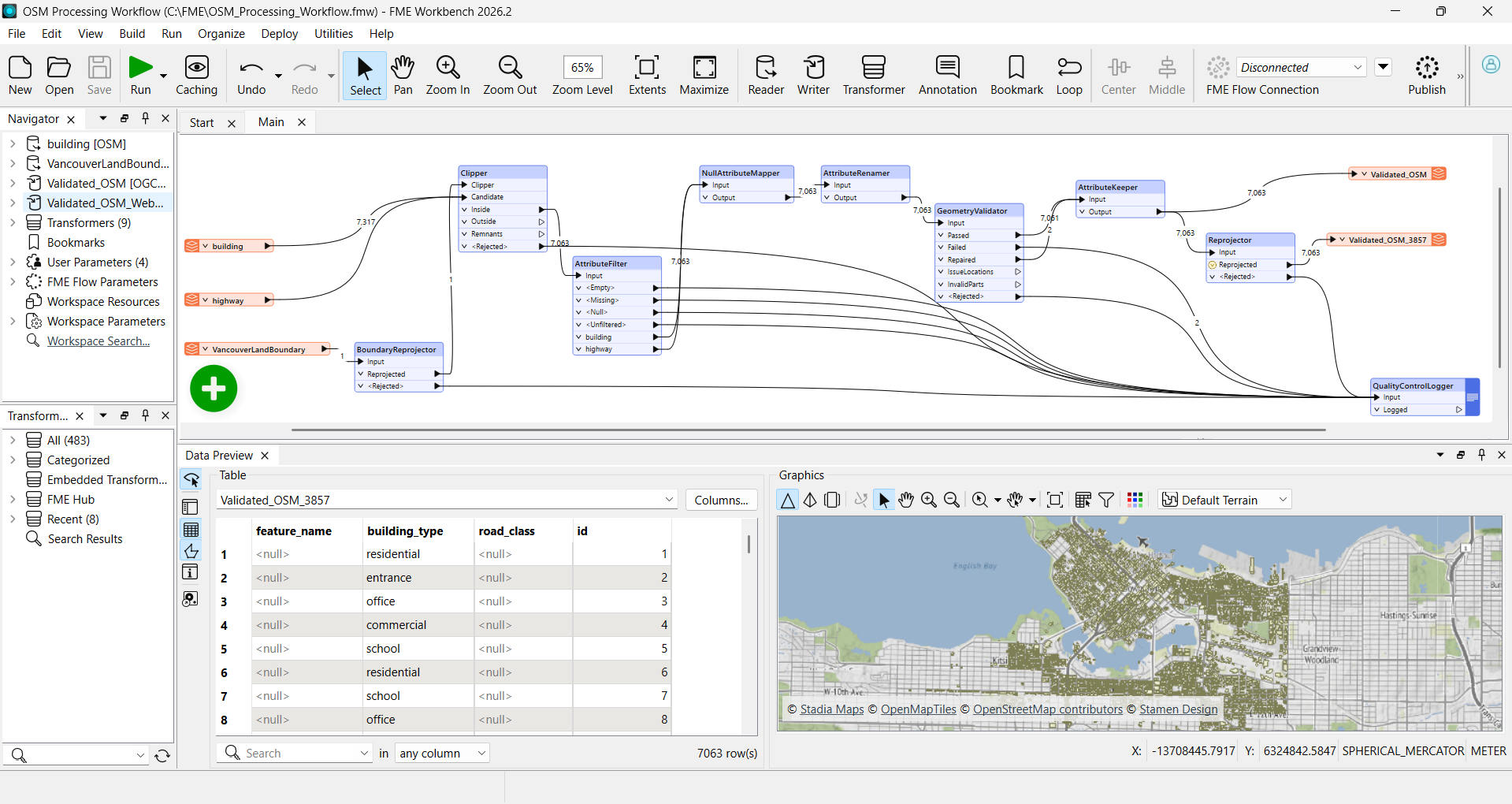
To add a Clipper transformer to limit the dataset to the exact area of interest, connect the city-boundary polygon to the Clipper input terminal and the OSM feature streams to the Candidate input terminal. Send the Inside output to the following stage and keep the Outside and <Rejected> outputs for quality control.

Step 3: Perform attribute filtering and cleaning

Apply an AttributeFilter to keep only those features that have meaningful classification tags—such as buildings that have a building tag or roads that have a highway tag indicating primary, secondary, or residential status—use a NullAttributeMapper to substitute null or empty values with appropriate defaults, and apply an AttributeRenamer to bring the field names in line with the target schema.

Learn how FME Realize automates spatial computing data processing

Watch WebinarWatch Webinar

Step 4: Validate and repair geometry

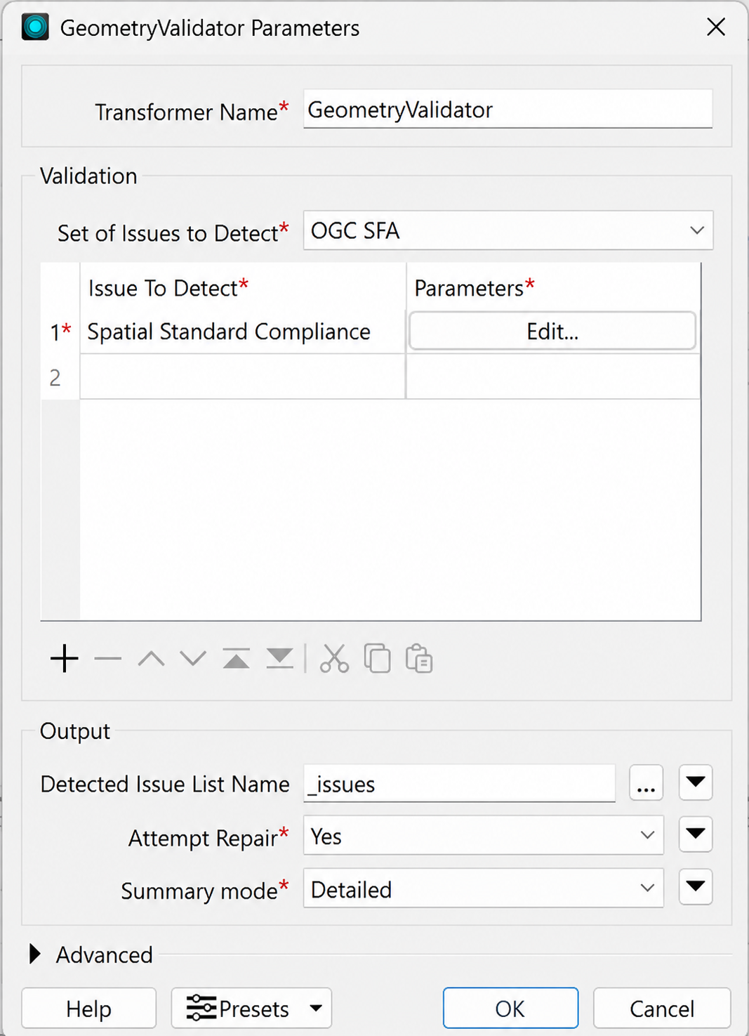
Add a GeometryValidator to pick up self-intersections, duplicate vertices, and other geometry errors. The transformer will automatically fix some of these errors each time the repair option is enabled. If snapping is required, use an AnchoredSnapper or a Snapper with a suitable tolerance. The features that still fail to be valid should be sent to a Logger or FeatureWriter for further examination and must not be included in the final output. This leads to a clear record of the valid features, those that have been repaired, and those that have been rejected.

In FME Workbench 2026.2, GeometryValidator provides predefined issue sets such as OGC SFA and can optionally repair detected geometry problems while producing detailed issue information.

Step 5: Confirm or reproject the CRS

Before adding a transformer, check the CRS of the source data. OpenStreetMap data is normally in WGS 84 (EPSG:4326), which is also the CRS used by KML, so no reprojection is needed when the source CRS is already defined correctly. If the coordinates are known to be in EPSG:4326 but the CRS information is missing, use a CoordinateSystemSetter to assign it. 

A Reprojector should only be used when the coordinate values need to be transformed. For example, separate outputs can be created in EPSG:27700 for British National Grid analysis or EPSG:3857 for web mapping, while the KML output remains in EPSG:4326.

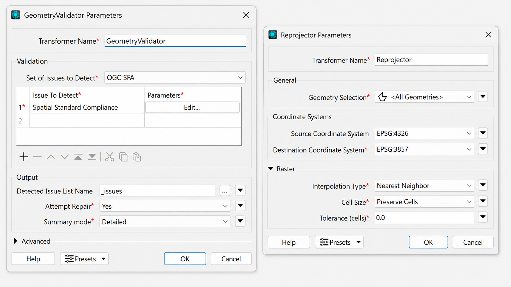
The parameter configuration of the principal validation and reprojection transformers is shown below.

Step 6: Write to KML

Include a KML writer, set the names of the output layers, define the style rules (using FME’s KML styling parameters to determine the colors, icon types, and line widths according to attribute values), specify the path for the output file, and then run the workspace. FME will generate a valid, georeferenced .kml file which can be opened directly in Google Earth, imported into Google Maps, or served via a downstream web map.

Since each reader, transformer, and writer is made up of parameters rather than being hard-coded, the only thing that needs to be changed to run the same workspace in a different city is the input extract, which means the pipeline can be reused.

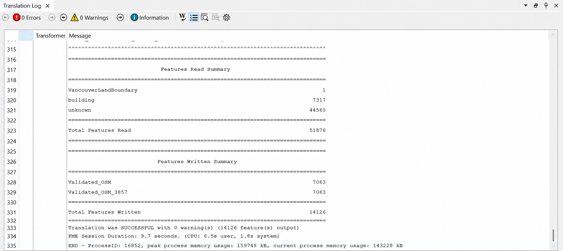
The following Translation Log excerpt summarizes the outputs and successful execution of the workspace in FME Workbench 2026.2. When performance profiling is enabled, FME also places a link to the resulting CSV report near the end of the log.

The completed pipeline will look as follows.

Best practices

The following best practices represent the core principles for building reliable, scalable, and maintainable geospatial data pipelines. Each practice addresses a specific class of risk encountered in production geospatial workflows.

Automate coordinate validation

When the data is ingested, the system should reject any coordinates that are outside the expected range or that appear suspicious, for example, those equal to 0,0, since they may lead to inaccurate outcomes in proximity analysis and spatial joins. In FME, the CoordinateSystemExtractor can display the assigned CRS, and the BoundsExtractor and Tester can verify if the data lies within the anticipated area. Any records that have missing or unexpected CRS information or contain invalid coordinates should be sent to a quarantine file for inspection. The CoordinateSystemSetter is used only when the correct CRS is known but has not yet been assigned, while the Reprojector is used when it is necessary to transform the coordinates.

Use a unified coordinate reference system

An effective governance decision in an organization is to designate a single coordinate reference system and enforce it at every stage of the data pipeline. This entails reprojecting data once at ingestion and asserting the target CRS at every pipeline output to prevent non-compliant data from reaching downstream consumers. In FME, the Reprojector transformer handles the conversion.

Make use of spatial autocorrelation

A basic assumption of ordinary least squares (OLS) regression is that the model errors are independent; however, this assumption may be invalid when dealing with geospatial data since values at nearby locations tend to be related. This aligns with Tobler’s First Law of Geography, which asserts that things that are near each other are generally more closely related than things that are far apart.

Spatial autocorrelation describes how values are distributed over space: positive autocorrelation indicates that similar values tend to be grouped, and negative autocorrelation shows that neighboring values are more different from each other. A value near zero suggests that there is little spatial pattern at the scale being examined. Moran’s I and Geary’s C are the methods most often used to assess this kind of relationship. In FME Workbench, residuals can be handled using PythonCaller with PySAL or RCaller with spdep or spatialreg. The statistics and p-value obtained in this way can be returned as feature attributes and then evaluated using a Tester before the workspace proceeds. Where the residuals reveal significant spatial dependence, a spatial lag or spatial error model might be more appropriate than ordinary least squares (OLS). GWR is used to deal with relationships that vary from one location to another, while kriging is applied for spatial interpolation; neither method can be used as a straightforward replacement for OLS merely because autocorrelation is present.

Like this article? Subscribe to our LinkedIn Newsletter to receive more educational content.

Subscribe NowSubscribe Now

Perform dynamic schema mapping

A pipeline that depends on fixed field names may stop working when a supplier changes a column name or data type. At runtime, the incoming schema should be checked against an approved schema before processing continues. In FME, SchemaScanner can be used to inspect attribute names and data types, while SchemaMapper can apply approved field renaming and value conversions using a mapping table. Unexpected fields and schema versions should be logged for review instead of being matched automatically. AttributeExposer can make hidden or dynamically created attributes visible in FME Workbench, but it does not perform fuzzy matching or schema mapping.

Optimize performance with data caching and data holding

To ensure that geospatial workflows are reliable, it is necessary to select the right data model, establish clear CRS and schema controls, carry out geometry and attribute validation, and use analytical methods that take into account spatial relationships. While FME can help make these steps easier to repeat and audit through a visual workspace, the user has to decide on the appropriate transformers, record the assumptions, and check the outputs. Once these practices are followed, geospatial data can be treated as a consistent information resource and used to support planning, logistics, environmental monitoring, and business decisions.

Conclusion

Geospatial data has shifted from being the concern of specialist cartographers to playing a central role in today’s data-driven organizations. The capacity to assign a location context to any event, asset, or transaction and to think spatially about patterns, relationships, and risk is, in fact, a real source of competitive and operational advantage.