Geographic Data
Geographic data describes objects, events, or conditions associated with locations on or near Earth’s surface. Although the terms “geographic data” and “spatial data” are often used interchangeably, spatial data can also refer more broadly to representations of physical, built, or virtual spaces. Geographic data typically combines coordinates, addresses, or named areas with geometry, attributes, and a coordinate reference system (CRS). These components make the spatial relationships in geographic data computable. Applications can calculate distances, test intersections, plan routes, and uncover patterns that ordinary database queries on simple relational data would miss.
Reliable analysis of geographic data depends on the accuracy of those references. Coordinates without a CRS are ambiguous; datasets captured at different scales may not align in an integration or conversion task. The end result may be a polished map that hides serious inconsistencies between source datasets.
This article explores data models, file formats, integration challenges, and best practices for geographic data workflows. It also features a hands-on example that compares a traditional Python pipeline with a modern, no-code automated workflow for a common industry task: converting CAD files into GIS data.
Summary of key geographic data concepts
| Concept | Description |
|---|---|
| What is geographic data? | Geographic data pairs earth-based locations with descriptive attributes. To be usable and consistently interpreted, this spatial data must include reference metadata like coordinate systems, units, and timestamps where relevant. |
| Core components of geographic data | Geographic data is more than location. Its geometry, descriptive attributes, identifiers, CRS and datum, scale or resolution, spatial relationships, temporal validity, and metadata determine what it represents and how it can be used. Missing or incorrect information may not stop the file from opening, but it can make the analysis misleading. |
| Models, formats, and storage | Geographic data relies on three core models: vectors for distinct features, rasters for continuous grids, and point clouds for 3D mapping. Geocoded data, which links addresses or place names to geographic coordinates, is commonly represented as vector points. The right format and storage method depend entirely on your access needs, scaling from simple files like GeoJSON and cloud-optimized formats like COG to robust spatial databases and APIs. |
| Common challenges when working with geographic data | Geographic data integration requires reconciling CRSes, datums, schemas, identifiers, geometry types, scale, accuracy, topology, update dates, and licensing. Large datasets also need indexing, partitioning, and tiling as well as repeatable quality checks. |
| Geographic data best practices | Define the target model before transforming data; preserve raw inputs; normalize reference systems and semantics explicitly; validate geometry, topology, attributes, and position; automate reruns; and record lineage, freshness, ownership, and restrictions. |
Understanding geographic data
A geographic dataset is more than just a set of coordinates. It combines location, descriptive attributes (e.g., location name, description, or land use), and reference information that explains how the data relates to the Earth. These components can be organized through different data models and stored or shared using various file formats, databases, and services. Understanding these elements provides the foundation for working with geographic data effectively.
Core components of geographic data
Here are the most important data components:
- Location and geometry: A feature may be represented as a point, line, polygon, multi-geometry, raster cell, pixel, or sampled 3D position. Note that geometry describes shape and position; it does not explain what the feature means.
- Attributes and identifiers: Names, categories, measurements, source IDs, and business keys give spatial features meaning and connect them to non-geographic systems. Stable identifiers are especially important for matching records across recurring updates. For example, in a relational database of cities, a primary key uniquely identifies each city, while foreign keys connect each to related records, such as country or administrative region.
- Coordinate reference system and datum: Coordinates are ambiguous without Earth-referencing rules. Geographic CRSes express angular coordinates; projected CRSes use linear units for a defined area. Datum transformations, units, and axis order must be handled explicitly.
- Scale, resolution, and accuracy: Map scale, raster cell size, collection method, positional accuracy, and degree of generalization determine which questions the data can reliably answer. For example, coordinates collected with a positional accuracy of 10 meters do not become more accurate when stored with six decimal places.
- Topology and spatial relationships: Containment, adjacency, connectivity, overlap, and proximity can be data requirements. Disconnected roads or overlapping districts may invalidate an analysis even when every coordinate is syntactically valid.
- Time, provenance, and metadata: Geographic data often comes with metadata that can describe when it was collected, the period for which it is valid, where it originated, how it was processed, and which licenses, restrictions, and ownership conditions apply. This information helps determine whether the data are current, auditable, and reusable.
Geographic data models
The following models are in widespread use:
- Vector data represents discrete features as points, lines, and polygons, including assets, roads, parcels, and boundaries. Multi-part geometries allow one logical record to contain several geometry parts.
- Raster data represents space as a grid for imagery, elevation, weather, land cover, and model outputs. Cell size, alignment, extent, and the meaning of each pixel are central to interpretation. Unlike vector data, raster data uses grid cells rather than discrete points, lines, and polygons.
- Point clouds and 3D data represent sampled surfaces as dense XYZ positions with attributes such as intensity, classification, timestamp, or color. LiDAR and photogrammetry are common sources.
- Geocoded tabular data in CSV files containing coordinates, addresses, postcodes, or area codes becomes geographic data when those references are interpreted and linked to locations with known quality and reference rules.
Formats, databases, and services
Here are some important technologies to understand:
- Geographic JavaScript Object Notation (GeoJSON): A simple, web-friendly format for points, lines, and areas. It uses World Geodetic System 1984 (WGS 84) longitude and latitude, so other coordinate systems may need conversion.
- GeoPackage: A portable file for vector data, map tiles, and related information. It follows an Open Geospatial Consortium (OGC) standard and is practical for sharing data.
- Geographic Tag Image File Format (GeoTIFF) and Cloud Optimized GeoTIFF (COG): GeoTIFF stores grid-based map data, while a COG allows online tools to load only the area and detail they need.
- GeoParquet: A format for analyzing and sharing large geographic datasets, especially through cloud platforms and compatible data tools.
- Shapefile: An older, widely supported vector format. It requires several companion files and has important limits, so use it mainly for compatibility with older systems.
- Spatial databases and application programming interfaces (APIs): PostGIS adds mapping capabilities to PostgreSQL. For example, services that follow the Open Geospatial Consortium (OGC) API Features standard let you request only the data you need, rather than downloading everything.
Challenges in working with geographic data
When setting up a geographic data pipeline, your data passes through several stages: ingestion, conversion, transformation, integration, analysis, and publication. Each stage brings its own challenges and can introduce errors into your geographic data pipeline. For example, a file may be technically valid while still using the wrong CRS, geometry, scale, schema, or date, yet still look convincing on a map.
A problem may remain hidden until the results are presented to stakeholders or used to support a decision. For that reason, reliable workflows need explicit assumptions, repeatable processes, and quality checks at every stage.
Here are some of the specific challenges that arise when working with geographic data:
- CRS, datum, and axis-order mismatch: Coordinates that look plausible may be interpreted in the wrong CRS, use another datum, swap latitude and longitude, or mix degrees with meters or feet. Reprojection must start from verified source metadata and an appropriate transformation; assigning a target CRS label to unchanged numbers is not reprojection.
- Format, schema, and semantic fragmentation: Sources may encode the same feature in CSV, GeoJSON, XML, GeoPackage, CAD, or a database with different field names, data types, categories, null conventions, geometries, or units. Reading bytes is usually easier than agreeing on meaning.
- Scale, resolution, and positional accuracy: Detailed municipal data may not align with a generalized national boundary, and a 10-meter raster cannot support parcel-level conclusions. Integration rules should respect the least precise source and the intended analysis.
- Geometry and topology defects: Self-intersections, empty geometries, duplicate vertices, polygon gaps or overlaps, disconnected roads, and out-of-area features can break analysis. Validation should distinguish safe, deterministic repairs from records that require review.
- Identifiers, duplicates, and entity resolution: Provider IDs may be missing, reused, or unique only inside one source. The same asset may appear with slightly different coordinates and attributes. To avoid problems, define canonical keys, matching tolerances, source precedence, and review rules instead of treating proximity alone as identity.
- Temporal mismatch and version drift: Boundaries, addresses, roads, and assets change. Sources collected on different dates can contradict one another in ways that look like spatial errors. Pipelines need effective dates, snapshots, incremental update rules, and a reproducible way to rebuild earlier outputs.
- Volume and performance: Large rasters, point clouds, and national feature datasets cannot always be loaded into memory or scanned repeatedly. Spatial indexes, bounding-box filters, partitioning, tiling, streaming, and cloud-optimized formats are design requirements, not late-stage tuning.
- Silos, governance, and sensitive locations: GIS desktops, field apps, databases, APIs, cloud storage, and legacy shares can hold conflicting copies. Teams must identify authoritative sources and control licensing, access, retention, publication, and sensitive-location handling.
- Cross-disciplinary expertise: Reliable geographic projects combine GIS expertise and domain judgement with data and software engineering. Data and software engineers provide the technical support needed to build, integrate, and maintain pipelines and applications. Depending on your project requirements, modern visual extract, transform, and load (ETL) tools can reduce the amount of custom code required, but production pipelines may still need engineering expertise.
Working with geographic data: Manual coding vs. modern visual ETL
Geographic data often moves between formats and systems before it can support analysis or operations. CAD-to-GIS conversion is common, particularly for public authorities that receive engineering drawings from planners, developers, and contractors. This CAD-to-GIS conversion is used in permitting, urban planning, utility and transport projects, and infrastructure asset management, where CAD designs must be aligned with authoritative geographic records.
In the following tutorial, we compare two ways to build the same workflow:
- A Python workflow, where the conversion logic is written directly in code using libraries such as ezdxf, Shapely, GeoPandas, and Pyogrio.
- A visual workflow, built in FME Workbench, Safe Software’s visual data-integration application, with the same logic configured through a user interface rather than code.
The task here is to convert a supplied CAD file (city_site_plan.dxf) into a GeoPackage containing building footprints. A specific layer (BUILDINGS) within the CAD file contains two nearly closed 2D polyline outlines. Because CAD files often lack reliable CRS metadata, EPSG:2227 was confirmed from the project documentation supplied with the DXF rather than derived automatically from the file. The target workflow closes small endpoint gaps, creates valid polygons, sets the source CRS to EPSG:2227, and reprojects the geometry to EPSG:4326.
In both approaches, the workflow follows the same four logical stages:
- Read the DXF and select the BUILDINGS features.
- Close endpoint gaps and construct valid polygons.
- Reproject the geometry from EPSG:2227 to EPSG:4326.
- Write the resulting building footprints to a GeoPackage.
Python expresses these stages in code, whereas FME represents them as connected workspace objects.
Here’s how the steps look at a conceptual level:
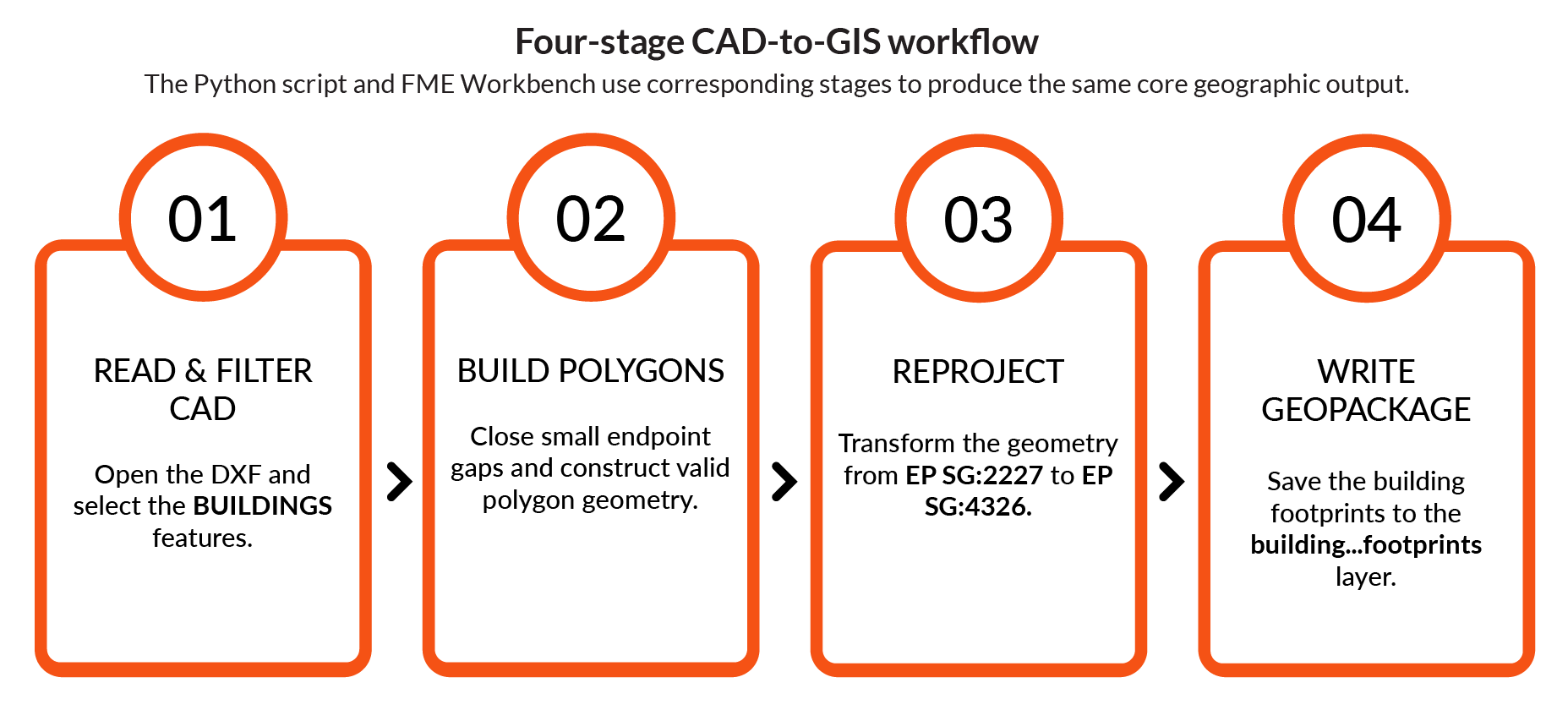
The point of comparing Python and FME Workbench is practical: A visual workflow reduces the need for specialized scripting skills and makes the pipeline easier for GIS professionals and other users to inspect. Python provides direct control over every rule, but it also requires programming knowledge and ongoing maintenance of the code and its dependencies.
If you want to locally reproduce this workflow, download the input CAD file and place it inside an “input” folder so that it is reachable at the relative path “input/city_site_plan.dxf”.
The traditional method: a Python script
To follow this Python tutorial, you’ll have to be familiar with basic Python functions, JSON handling, and relevant command-line tools.
The supplied script uses the ezdxf Python module for CAD access, Shapely for geometry construction and repair, GeoPandas for the feature table and reprojection, and Pyogrio for GeoPackage output.
Before starting, you need to install dependencies as follows: python -m pip install ezdxf geopandas shapely pyogrio.
Let’s get into the code. The first block of Python code imports the required libraries and fixes the workflow contract: input and output paths, layer name, source and target CRSs, and the maximum endpoint gap. These constants make the assumptions reviewable before any geometry is changed.
from math import dist
from pathlib import Path

import ezdxf
import geopandas as gpd
from shapely.geometry import MultiPolygon, Polygon
from shapely.validation import make_valid


INPUT_CAD = Path("input/city_site_plan.dxf")
OUTPUT_GPKG = Path("output/city_buildings.gpkg")
OUTPUT_LAYER = "building_footprints"
SOURCE_CRS = "EPSG:2227"
TARGET_CRS = "EPSG:4326"
MAX_GAP_FT = 0.01In the next Python code block, we introduce helper functions. They are used to isolate geometry-specific rules. For instance, polygon_parts() extracts polygon members from the result of make_valid(). Then the function repair_outline() rejects outlines with fewer than three vertices and rejects bulged arc segments because they would need tessellation. It then checks the endpoint gap. When the gap is within MAX_GAP_FT, the final coordinate is replaced with the first to snap the endpoints together.
Replacing rather than appending the coordinate creates an explicitly closed ring without retaining a near-duplicate vertex and a very short closing segment. Larger gaps are rejected to avoid closing a potentially intentional opening. The function then repairs invalid geometry and returns all valid polygon parts as a MultiPolygon with diagnostics.
def polygon_parts(geometry):
 	"""Extract every polygon from repaired Shapely geometry."""
 	if geometry.geom_type == "Polygon":
     	return [geometry]
 	if hasattr(geometry, "geoms"):
     	return [part for child in geometry.geoms for part in polygon_parts(child)]
 	return []
def repair_outline(entity):
"""Close one nearly closed CAD outline and return valid polygon geometry."""
vertices = list(entity.get_points("xyb"))
if len(vertices) < 3:
raise ValueError("fewer than three vertices")
if any(abs(float(vertex[2])) > 0 for vertex in vertices):
raise ValueError("contains a bulged arc; tessellation is required")
coordinates = [(float(x), float(y)) for x, y, _ in vertices]
if entity.closed:
gap = 0.0
if coordinates[-1] != coordinates[0]:
coordinates.append(coordinates[0])
else:
gap = dist(coordinates[0], coordinates[-1])
if gap > MAX_GAP_FT:
raise ValueError(f"endpoint gap is {gap:.3f} ft")
coordinates[-1] = coordinates[0]
candidate = Polygon(coordinates)
parts = polygon_parts(make_valid(candidate))
if not parts:
raise ValueError("geometry repair produced no polygon")
return MultiPolygon(parts), gap, gap > 0 or not candidate.is_validNext, we introduce the main part of the Python code, which works in four steps, as shared in the introductory part of this section.
Step 1 opens the DXF and queries only LWPOLYLINE entities on BUILDINGS.
Step 2 processes each CAD entity independently, preserving its handle and layer while recording gap_ft and was_repaired. A repair failure is printed with the CAD handle and skipped; if every candidate fails, the pipeline stops rather than publishing an empty success.
Here’s the code for the first two steps.
# STEP 1 READER: Open the DXF and select BUILDINGS polylines.
 if not INPUT_CAD.exists():
 	raise FileNotFoundError(f"Input not found: {INPUT_CAD.resolve()}")
 drawing = ezdxf.readfile(INPUT_CAD)
 building_lines = drawing.modelspace().query('LWPOLYLINE[layer=="BUILDINGS"]')


 # STEP 2 AREA BUILDER: Close small gaps, validate outlines, and make polygons.
 features = []
 for entity in building_lines:
 	handle = entity.dxf.handle or "unknown"
 	try:
     	geometry, gap, was_repaired = repair_outline(entity)
     	features.append({"cad_handle": handle, "cad_layer": "BUILDINGS",
                      	"gap_ft": gap, "was_repaired": was_repaired,
                      	"geometry": geometry})
 	except ValueError as error:
     	print(f"Skipped CAD handle {handle}: {error}")
 if not features:
raise RuntimeError("No usable building footprints were produced.")Step 3 is the point where the cleaned spatial shapes are made explicitly geographic. GeoPandas is told that the existing numbers use EPSG:2227, then to_crs() calculates new coordinates in EPSG:4326. Assigning EPSG:4326 directly to the original State Plane numbers would only relabel them and would place the features incorrectly.
# STEP 3 REPROJECTOR: Assign EPSG:2227, then transform coordinates to EPSG:4326.
 buildings = gpd.GeoDataFrame(features, geometry="geometry", crs=SOURCE_CRS)
buildings = buildings.to_crs(TARGET_CRS)Step 4 creates the output directory, removes any existing demonstration file, and writes the `building_footprints` layer using the GeoPackage driver. Removing the previous output ensures that each tutorial run starts from the same state. Production pipelines should instead use explicit overwrite or versioning rules to prevent accidental data loss.
# STEP 4 WRITER: Replace the old output and write the GeoPackage to disk.
 OUTPUT_GPKG.parent.mkdir(parents=True, exist_ok=True)
 if OUTPUT_GPKG.exists():
 	OUTPUT_GPKG.unlink()
 buildings.to_file(OUTPUT_GPKG, layer=OUTPUT_LAYER, driver="GPKG",
               	engine="pyogrio", index=False)
print(f"Wrote {len(buildings)} features to {OUTPUT_GPKG}:{OUTPUT_LAYER}")For the supplied DXF, a successful run writes two features.
If the Python script runs successfully, then you should see the following printout in your command prompt or IDE:
Wrote 2 features to output/city_buildings.gpkg:building_footprintsIf you’ve worked with geographic data before, none of those individual operations or steps should be unusual for you. The engineering challenge comes from combining these four steps into a dependable pipeline while keeping the Python environment and native geospatial dependencies stable.
Keep in mind that this Python script is intentionally narrow. It supports only straight, two-dimensional lightweight polyline entities; bulged segments, blocks, hatches, dimensions, three-dimensional (3D) entities, and variations in contractor layer conventions fall outside its scope. In a real-world project, this approach would require additional parsing and tests, clear rules for handling failures, and ongoing maintenance as CAD conventions evolve.
The visual workflow: FME Workbench
FME is a low-code spatial data integration platform with a flat learning curve that enables even non-programmers to handle geospatial data. The same CAD-to-GIS conversion that we showed above can be built as a visual workflow in FME Workbench.
The following procedure reflects the tested configuration in FME Workbench 2026.1 and follows the same four logical steps as the Python approach:
- Read the DXF and select the `BUILDINGS` features.
- Close the endpoint gaps and construct polygons.
- Reproject the polygons from EPSG:2227 to EPSG:4326.
- Write the building footprints to a GeoPackage.
Before starting, place the correct input CAD file in the project’s “input” folder and create a writable “output” folder.
The completed feature flow is:
BUILDINGS reader feature type → AreaBuilder Area → Reprojector Reprojected → building_footprints writer feature type
Here’s a detailed breakdown of each step in the CAD-to-GIS process:
Step 1: Read and filter the CAD data
First, add the Reader. Select “Reader” on the toolbar, or choose “Readers” and then “Add Reader”.

Then, select the input format and dataset. Set Format to Autodesk AutoCAD DWG/DXF and browse to “input\city_site_plan.dxf”.
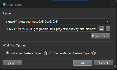
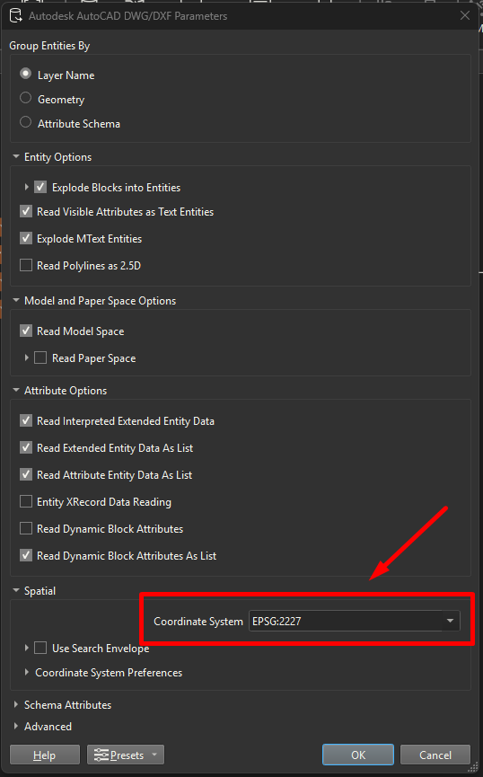
Next, assign the source coordinate system. Set the coordinate system to EPSG:2227.
When done with the coordinate system configuration, move on to the Reader parameters. Use the following settings:
- Read Polylines as 2.5D: No
- Read Model Space: Yes
- Read Paper Space: No
The configuration of the reader should look like this:
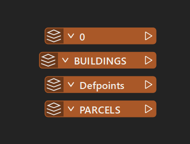
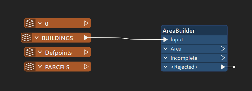
After clicking OK and adding the reader, FME generates the reader feature types; confirm that `0`, `BUILDINGS`, `Defpoints`, and `PARCELS` appear on the canvas.
You will only need `BUILDINGS` to be connected to AreaBuilder; we’ll show how to set it up in Step 2.
Step 2: Close the endpoint gaps and construct polygons
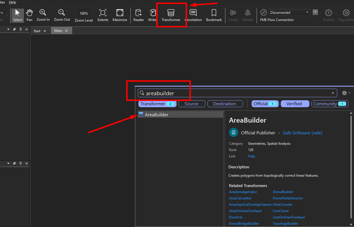
Drag an AreaBuilder from the Transformer Gallery onto the canvas.
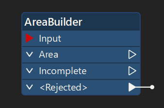
It should appear as follows:
Next, connect the `BUILDINGS` reader output to AreaBuilder’s Input port.
Open the AreaBuilder parameters. Under Snapping Pre-Processing, choose End Point Snapping and set Snapping Tolerance to “0.01” (U.S. survey feet, the ground units of EPSG:2227).
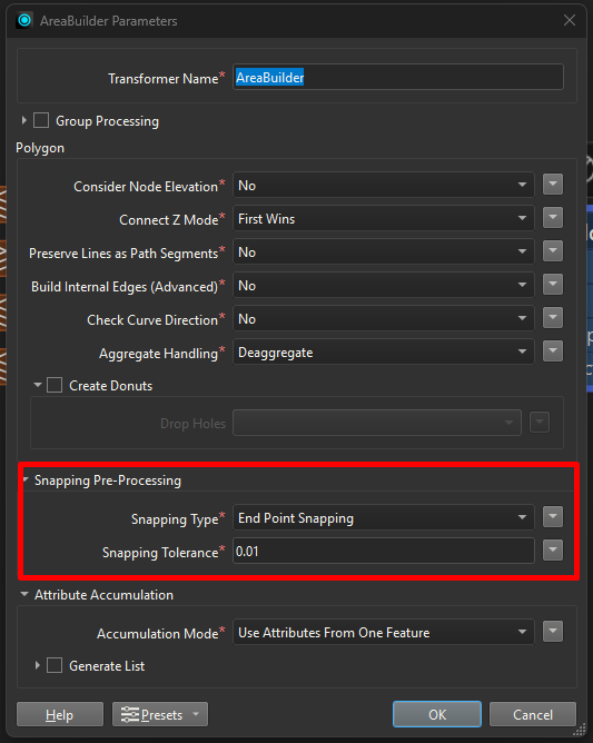
As you may notice in the provided screenshot, the following settings were used:
- Group Processing / Group By: Disabled or blank
- Consider Node Elevation: No
- Connect Z Mode: First Wins
- Preserve Lines as Path Segments: No
- Build Internal Edges: No
- Check Curve Direction: No
- Aggregate Handling: Deaggregate
- Create Donuts: Unchecked
- Drop Holes: No
- Attribute Accumulation Mode: Use Attributes From One Feature
- Generate List: Unchecked
Step 3: Reproject the polygons
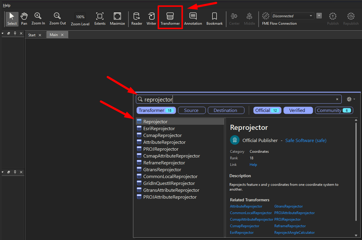
Start the third step by placing a Reprojector to the right of AreaBuilder. First, select a Reprojector feature from the Transformers menu.
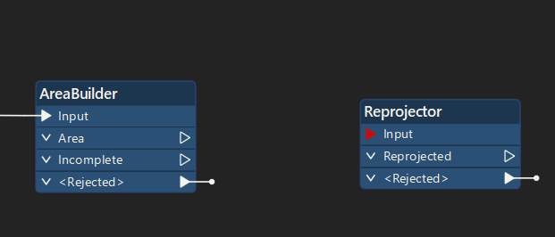
It should appear like this, next to the AreaBuilder.
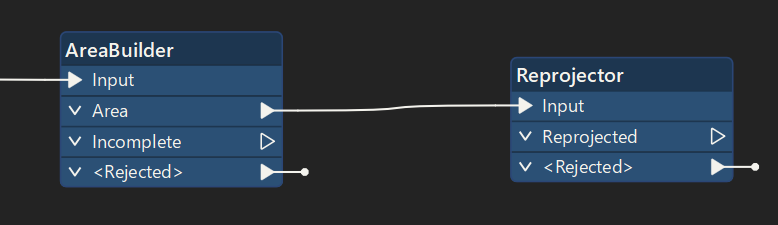
Then connect AreaBuilder: Area to Reprojector: Input port.
Configure the Reprojector parameters. Leave Source Coordinate System set to <Read from geometry>.
The polygons already carry EPSG:2227 from the Reader. Set Destination Coordinate System to LL84.
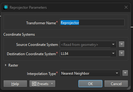
The displayed Raster Interpolation Type can remain Nearest Neighbour.
Step 4: Write the building footprints to a GeoPackage
The fourth step is the last one. Start by selecting the Writer on the toolbar and choosing OGC GeoPackage as the format. Set Dataset to “output\city_buildings_FME.gpkg” and change Table Definition from Automatic to Manual.
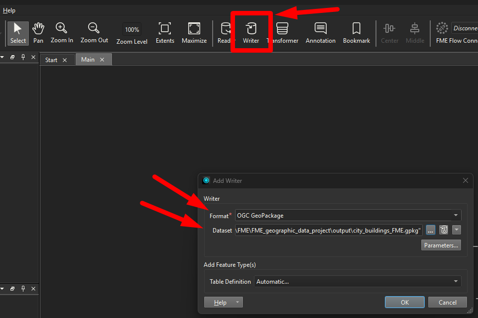
Configure the dataset-level parameters. Use the following settings:
- Overwrite Existing Database: Yes,
- Template File: Blank,
- Version: 1.3,
- Feature Type Names case: None,
- Attribute Names case: None.
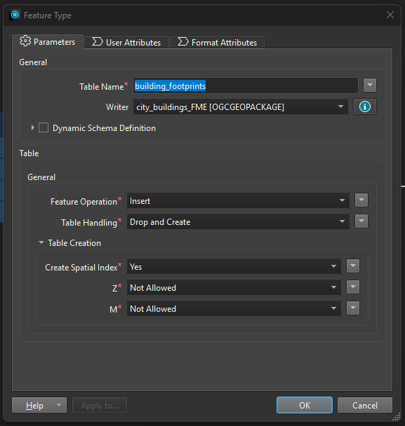
Next, in the configuration window that pops up, replace the default table name “Table1” with “building_footprints”. Set the schema and write behavior.
You can leave Dynamic Schema Definition unchecked, set Feature Operation to Insert, and set Table Handling to Drop and Create. Configure the output geometry.
You will also need to expand “Table Creation” and use the following values:
- Geometry: `geopackage_polygon`
- Geometry Column: `geom`
- Create Spatial Index: Yes
- Z: Not Allowed
- M: Not Allowed
Here’s how it should look:
Finally, connect Reprojector: Reprojected to “building_footprints”.
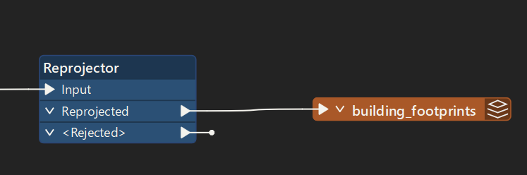
And now your FME Workbench workspace is ready to run. You do so by clicking the green arrow in the upper left corner. The expected result is two polygon features written to the “building_footprints” table in “city_buildings_FME.gpkg”.
Here is how the full workflow looks on the FME Workbench Canvas:

The input CAD file (i.e., DXF) also contains feature types named `0`, `Defpoints`, and `PARCELS`. Leave these unconnected because they are not part of the CAD design that we want to convert to GIS.
In the bigger picture, the FME and Python workflows achieve the same business objective and produce the same core geographic result. They both read the same CAD layer, close the two small endpoint gaps, construct valid polygons, and transform them from EPSG:2227 to WGS 84. FME specifies this destination as LL84, while the Python workflow uses EPSG:4326. Both represent WGS 84 geographic coordinates in degrees; LL84 follows the conventional longitude/latitude (x/y) order, while GeoPandas handles EPSG:4326’s formal latitude/longitude axis order internally.
After this processing is completed, both approaches write the result to the hard drive as a GeoPackage.
Recommendations and best practices
Here are some best practices for your next geographic data project:
- Define the target question and model first: Decide which decisions, joins, measurements, and systems the output must support. Specify geometry type, CRS, fields, identifiers, units, null rules, time, and quality thresholds before mapping source data.
- Treat CRS metadata as required data: Verify the source CRS and datum at ingestion, preserve the original reference, apply a transform with an explicit operation, and test on a known location. Never repair a mismatch by assigning the desired CRS to unchanged coordinate numbers.
- Preserve raw inputs and make transformations reproducible: Keep immutable snapshots or versioned references. Separate raw, normalized, and published layers so outputs can be rebuilt and corrections traced to a rule rather than to an undocumented desktop edit.
- Standardize semantics and identifiers early: Normalize field names, types, categories, units, and missing values near the start of the pipeline. Retain source IDs alongside canonical IDs and document matching, tolerance, source-precedence, and conflict-resolution rules.
- Validate geometry, topology, attributes, and position: Use quality gates for valid, expected geometry; coordinate ranges; required attributes; uniqueness; topology; containment; and domain rules. Route failures to a review output instead of silently dropping them or auto-fixing every record.
- Choose storage for the access pattern: Use GeoJSON for modest web interchange, GeoPackage for portable multi-layer exchange, GeoTIFF or COG for rasters, GeoParquet for analytical feature data, and a spatial database when concurrent queries, governance, and controlled updates matter.
- Design for scale before volume forces a rewrite: Filter by bounds and attributes early, use spatial indexes, partition or tile large datasets, stream where possible, and avoid unnecessary reprojection or serialization. Benchmark representative geometry complexity rather than file size alone.
- Automate updates, lineage, and safeguards: Make reruns idempotent while recording source versions, checkpoints, tests, logs, ownership, and freshness. AI can assist with documentation or proposed schema mappings, but geographic transformations, validation, and sensitive-location decisions should remain deterministic and reviewable.
Last thoughts
Geographic data involves more than sets of coordinates and descriptions. A reliable dataset should also state its coordinate system, units, level of detail, date, source, processing history, and known limits. In a decision-support context or a consulting project, this information indicates which measurements, comparisons, and decisions can be trusted. A file can look correct on a map and still be unsuitable for analysis.
The CAD-to-GIS conversion example shows why. The source outlines start as simple shapes. They become useful geographic data after their coordinate system is confirmed, errors are fixed, coordinates are converted, and results are checked.
Both Python and FME Workbench can convert CAD files into GIS formats; the right choice depends on the team’s skills, project needs, and budget. Regardless of the tool you choose, your team should follow established best practices. A detailed list appears earlier in this article, but three practices deserve particular emphasis: recording where the data came from, explaining how errors are handled, and documenting the decisions made.
Continue reading this series
Spatial Computing
Learn the basics of spatial computing and its benefits, key applications, and practical examples for processing spatial data using low-code frameworks like FME and traditional GIS software.
KML To GeoJSON
Learn about converting KML to GeoJSON files, including methods, best practices, and key differences between the two spatial file formats.
Geospatial Data Integration: Best Practices
Learn about the importance of seamless integration of diverse geospatial data sources and the challenges, best practices, and workflows involved in achieving accurate mapping and analyses for decision-making.
Shapefile To GeoJSON: Best Practices
Learn three proven methods to convert shapefiles to GeoJSON for modern web mapping applications.
Digital Twin Examples
Learn how digital twin examples are reshaping manufacturing, cities, hospitals, and farms with real-time data.
Augmented Reality Databases
Learn the key database types, data requirements, and best practices for building production-ready augmented reality systems.
MCP Server Geospatial: Tutorial & Implementation
Learn how a geospatial MCP server connects AI agents to spatial tools reliably and at scale.
Spatial Data
Learn how spatial data models, formats, and no-code automation tools simplify complex integration workflows.
What is Geospatial Data
Learn geospatial data fundamentals, real-world use cases, pipeline implementation steps, and best practices using FME.
Digital Twins in Manufacturing
Learn what digital twins are, their manufacturing use cases, and how to tackle data integration challenges while digital twins effectively.
Digital Twins in Urban Planning
Learn how digital twins in urban planning enable real-time monitoring, scenario simulation, and smarter infrastructure decisions.
GeoPandas
Learn how GeoPandas loads, validates, and joins vector data in a complete point-in-polygon workflow.
Geographic Data
Learn what geographic data is, how it works, and best practices for managing spatial data workflows.
Visual Spatial Intelligence
Learn how production systems combine spatial data and geometry to answer real-world measurement questions reliably today.