GeoPandas
GeoPandas is a Python library that enhances pandas with geometry-aware data structures and spatial operations for vector geospatial data, making it essential for location-based data processing. It provides geometric data types and spatial computing capabilities, helping users perform spatial analysis workflows effectively.
In spatial computing, spatial datasets do not always contain a common attribute for a conventional join. When the relationship between two datasets depends on location, the connection must instead be derived from their geometries. GeoPandas is useful for these problems.
This article highlights a point-in-polygon example using a sample dataset. The workflow reads both point and polygon datasets, analyzes their metadata, geometry, and coordinate reference system (CRS), and performs a spatial join. The workflow further analyzes unmatched and multiple-match cases, counts points per polygon, reconciles totals, and writes the results to GeoJSON.
Summary of key GeoPandas concepts
| Concept | Description |
|---|---|
| GeoPandas data model | The GeoPandas data model uses DataFrames with a geometry column, allowing tabular and spatial attributes to coexist in a single vectorized data structure. |
| Spatial data and coordinate reference system (CRS) management | GeoPandas reads and writes geospatial data in various formats (Shapefile, GeoJSON, GeoPackage, etc.) using Fiona or Pyogrio. PyProj handles coordinate reference system transformations (such as CRS assignment and reprojection). |
| Geometry quality | GeoPandas validates geometry with basic tools for geometric integrity, helping identify and fix invalid polygons, self-intersections, and null geometries. |
| Spatial relationships | GeoPandas supports spatial relations (e.g., intersects, contains, and within) and overlay operations (e.g., union, difference, intersection) to analyze relationships among geographic features. |
| Interoperability and integration | GeoPandas can export data to web applications, GIS software, and spatial databases. It facilitates sharing data through formats like GeoJSON for web mapping. |
| Scaling and production workflows | Processing in memory involves careful resource management. For larger workflows, partitioning and processing on a database server are common practices. |
| Best practices for using GeoPandas | Best practices include optimizing performance by using spatial indexing for joins, filtering data early in the pipeline, validating geometries upfront before analysis, and avoiding expensive operations on unprojected geographic coordinates. |
Understanding the GeoPandas data model
How GeoPandas represents spatial data underpins spatial joins, changing defined coordinate reference systems (CRS), and verifying geometry. Each of these functions is dependent on GeoDataFrames and GeoSeries being interpreted correctly.
GeoPandas includes attribute data along with geometry and spatial metadata, organizing them into structures similar to Pandas objects. For example, a GeoDataFrame may hold a table of cities with a geometry column containing each city’s point location. In contrast, a GeoSeries may contain just those geometries as a single, spatially aware series. The geometry column stores the shapes used for spatial operations, and the CRS metadata records the coordinate reference system so that distances, joins, and transformations are interpreted correctly. This matters because all subsequent steps in the workflow (like spatial joins, geometry validation, CRS transformations, and aggregations) work with these structures.
Two structures in GeoPandas carry the spatial behavior:
- A GeoDataFrame is a pandas DataFrame that includes geometry.
- A GeoSeries is a one-dimensional column of geometry objects that can exist on its own or serve as a column inside a GeoDataFrame.
The individual values in a GeoSeries are Shapely geometry objects, which is why operations such as containment tests are available without writing coordinate arithmetic by hand.
Everything else in a GeoDataFrame is an ordinary attribute column. Identifiers, names, categories, and measurements behave exactly as in pandas, so the familiar groupby, merge, and fillna operations remain available.
Now that we understand the basics of the GeoPandas framework, we will shift focus to handling typical geospatial computing tasks. The following sections explain typical workflows for working with spatial data and how GeoPandas handles them.
Working with spatial data and CRS management
GeoPandas handles various spatial formats and CRS management, which is crucial for data interoperability and spatial accuracy. Using Pyogrio, Fiona, and Pyproj, it ensures that coordinate systems are correctly assigned and transformed, maintaining spatial logic throughout analysis workflows. Let’s see how it handles some typical workflows.
Loading and inspecting spatial data
GeoPandas reads most vector-based spatial data formats using the geopandas.read_file() function. It provides an interface for reading supported vector formats. The function uses Pyogrio or Fiona to access the appropriate GDAL/OGR driver and returns a GeoDataFrame.
In any code that depends on specific datasets, it is best to isolate dataset parameters from the reusable components. Be sure to group paths, field names, predicates, and output CRS within a configuration.
To avoid the uncertainty of external shapefiles, we will now create our own sample dataset, which will let us remove uncertainty in our spatial logic by letting us know exactly what to expect from our inspection methods.
from pathlib import Path
import geopandas as gpd
from shapely.geometry import Polygon, Point

# ------------------------------
# CONFIGURATION
# ------------------------------
PROJECT_DIR = Path("PROJECT_DIRECTORY")  # Users replace this
POLYGON_ID_FIELD = "POLYGON_ID"
POLYGON_NAME_FIELD = "POLYGON_NAME"
POINT_ID_FIELD = "POINT_ID"
JOIN_PREDICATE = "within"
WEB_OUTPUT_CRS = "EPSG:4326"

# ------------------------------
# SAMPLE DATA
# ------------------------------
# Create a simple administrative boundary (square) and points with specific edge cases.
polygon_features = gpd.GeoDataFrame(
    {
        POLYGON_ID_FIELD: [1, 2],
        POLYGON_NAME_FIELD: ["District A", "District B"],
        "geometry": [
            Polygon([(0, 0), (10, 0), (10, 10), (0, 10)]),  # Square A
            Polygon([(10, 0), (20, 0), (20, 10), (10, 10)]) # Square B
        ]
    },
    crs="EPSG:3857"  # Projected CRS for accurate distance
)

point_features = gpd.GeoDataFrame(
    {
        POINT_ID_FIELD: [1, 2, 3, 4, 5, 6, 7],
        "geometry": [
            Point(5, 5),
            Point(15, 5),
            Point(5, 10),
            Point(-1, 5),
            Point(10, 5),
            Point(2, 2),
            Point(12, 8)
        ]
    },
    crs="EPSG:3857"
)

# If users want to load their own files, they can replace the above with `gpd.read_file(POLYGON_PATH)` and `gpd.read_file(POINT_PATH)`.With the datasets loaded, inspect both of them:
print(polygon_features.head())
print(point_features.head())
print(polygon_features.columns)
print(point_features.columns)
print(polygon_features.total_bounds)
print(point_features.total_bounds)
print(polygon_features.crs)
print(point_features.crs)Applying these inspection methods to the GeoDataFrames reveals the data structure, geometry types, and coordinate reference systems. The output from the console is as follows:
# Print polygon_features.head()
   POLYGON_ID POLYGON_NAME                    geometry
0           1    District A  POLYGON ((0 0, 10 0, 10 10, 0 10))
1           2    District B  POLYGON ((10 0, 20 0, 20 10, 10 10))
# Print point_features.head()
   POINT_ID                  geometry
0         1      POINT (5 5)
1         2      POINT (15 5)
2         3      POINT (5 10)
3         4      POINT (-1 5)
4         5      POINT (10 5)
# Print polygon_features.columns
Index(['POLYGON_ID', 'POLYGON_NAME', 'geometry'], dtype='object')
# Print point_features.columns
Index(['POINT_ID', 'geometry'], dtype='object')
# Print polygon_features.total_bounds
[ 0.  0. 20. 10.]
# Print point_features.total_bounds
[-1.  2. 15. 10.]
# Print polygon_features.crs
EPSG:3857
# Print point_features.crs
EPSG:3857Next, review the available columns, layer bounds, and CRS metadata to detect missing metadata or spatial misalignment. Examine the bounds and CRS metadata to locate displaced layers. CRS metadata may also be absent.
Aligning coordinate reference systems
Coordinate reference systems establish the relationship between real-world locations and coordinate values. Ensuring CRS compatibility helps you trust your spatial relationships and builds confidence in your analysis.
if polygon_features.crs is None:
    raise ValueError("The polygon dataset does not have CRS metadata.")
if point_features.crs is None:
    raise ValueError("The point dataset does not have CRS metadata.")
points_aligned = point_features.to_crs(polygon_features.crs)You can perform a spatial join when both layers use a compatible CRS; use set_crs() when you want to assign CRS metadata without changing the coordinates. The to_crs() function changes coordinates to a new CRS altogether. Keep in mind that relabeling a layer to match another layer’s CRS metadata will allow the join to run but will place layer features in the wrong locations.
Checking geometry quality
Geometry quality describes whether a spatial feature has geometry and whether that geometry is of the appropriate type. A record can have no geometry, empty geometry, or invalid geometry (like a self-intersecting polygon). These are all geometry quality issues, but they represent different conditions and should be evaluated separately.
Point-in-polygon analysis uses geometry spatial predicates, which rely on the geometry quality of each involved spatial feature. Empty geometries can’t produce a meaningful match; geometry quality matters to the analysis. Invalid geometry may produce unforeseen spatial relationships. Because of this, the workflow checks geometry quality before the spatial join.
The only required attributes for the spatial comparison are the geometry, name, and polygon identifier. Thus, the active working layer is filtered to only those attributes:
polygon_boundaries = polygon_features[

    [POLYGON_ID_FIELD, POLYGON_NAME_FIELD, "geometry"]

].copy()The polygon and point layers can then be evaluated separately for missing, empty, and invalid geometries:
missing_polygon_geometry = (
    polygon_boundaries.geometry.isna()
)
empty_polygon_geometry = (
    polygon_boundaries.geometry.is_empty
)
invalid_polygon_geometry = (
    polygon_boundaries.geometry.notna()
    & ~empty_polygon_geometry
    & ~polygon_boundaries.geometry.is_valid
)
missing_point_geometry = (
    points_aligned.geometry.isna()
)
empty_point_geometry = (
    points_aligned.geometry.is_empty
)
invalid_point_geometry = (
    points_aligned.geometry.notna()
    & ~empty_point_geometry
    & ~points_aligned.geometry.is_valid
)

print("Missing polygon geometries:", missing_polygon_geometry.sum())
print("Empty polygon geometries:", empty_polygon_geometry.sum())
print("Invalid polygon geometries:", invalid_polygon_geometry.sum())

print("Missing point geometries:", missing_point_geometry.sum())
print("Empty point geometries:", empty_point_geometry.sum())
print("Invalid point geometries:", invalid_point_geometry.sum())Since we are using a clean sample dataset, we expect no missing, empty, or invalid geometries. This check confirms that the data is structurally ready for a spatial join. The output that follows serves as an initial baseline of quality:
Missing polygon geometries: 0
Empty polygon geometries: 0
Invalid polygon geometries: 0

Missing point geometries: 0
Empty point geometries: 0
Invalid point geometries: 0
Missing geometry means a record of a spatial attribute has no associated geometry. If a geometry has no coordinates, it is considered empty. If a geometry is a self-intersecting polygon ring, which violates the structuring rules of geometry, then it is invalid geometry. Distinguishing between these cases makes it easier to determine whether to repair, omit, or examine a feature further.
Invalid polygons may sometimes be repaired before analysis, although repair should be treated as a data-quality decision rather than an automatic step:
if invalid_polygon_geometry.any():
    polygon_boundaries.loc[
        invalid_polygon_geometry,
        "geometry",
    ] = (
        polygon_boundaries.loc[
            invalid_polygon_geometry,
            "geometry",
        ].make_valid()
    )

print(
    "Remaining invalid polygons:",
    (~polygon_boundaries.geometry.is_valid).sum(),
)

print("Polygon geometry types after repair:")
print(polygon_boundaries.geom_type.value_counts())If the Python script runs successfully, then you should see the following printout in your command prompt or IDE:
Remaining invalid polygons: 0make_valid() may generate a valid geometry type; multipart structures or GeometryCollections may be introduced. Following a make_valid() call, both the validity and type of geometry should be assessed to determine whether the new geometry type is valid for the join in question.
Understanding spatial relationships
Spatial relationships describe how geographic features interact based on geometry and location, not shared attributes. For example, a point can be inside a polygon, touch a polygon’s boundary, intersect a polygon, or be outside a polygon. In GeoPandas, these relationships are represented using spatial predicates such as within, contains, and intersects.
These predicates are critical because the chosen geometric relationship will establish which features are considered a match. For instance, a store point can be assigned to the administrative area polygon that contains it, even though the store and administrative polygons differ in all other attributes. Point geometry located on a polygon boundary may also behave differently depending on whether within or intersects is used in the analysis.
Performing a point-in-polygon spatial join
In this case, sjoin() is used to apply the desired predicate to assign each point to the appropriate polygon:
points_with_polygon = gpd.sjoin(

    points_aligned,

    polygon_boundaries,

    how="left",

    predicate=JOIN_PREDICATE,

)The point layer is on the left because the question being asked is about points: Each point should end up with the attributes of the polygon that contains it. That orientation also determines the shape of the result, which has one row per matched point rather than one row per polygon.
The parameter how=”left” retains all input records, matched or not. Points that fall outside the polygon’s coverage should be examined. To reconcile the output row count with the input count, the output must retain those points.
If JOIN_PREDICATE is set to within, it checks whether a point lies within a polygon. However, people are often surprised that points on a shared boundary (such as a coastline or the edge of an administrative polygon) are not “within” either polygon and thus will be unmatched. Switching to intersects includes boundary contact and will match those points and can match a single point to two adjacent polygons that share the edge. Neither predicate is more correct in general; the choice follows the business rule, and it is worth recording that rule alongside the code.
Investigating unmatched and multiple matches
The valid state of geometries and their coordinate reference systems does not guarantee that a spatial join will yield an unambiguous one-to-many relationship for the join subject. Some points may not match, and some may match multiple polygons. When applicable, these cases provide insight into the data and the spatial constraint being enforced.
For instance, a point that is located outside the study area should remain and, in fact, be unmatched. A point that falls exactly on the boundary line of two polygons may remain unmatched with respect to “within” but may also match both polygons with respect to “intersects.” Valid geometries can still yield multiple matches when polygons overlap.
Before aggregation, address these situations, as unmatched points may decrease totals while multiple matches may increase them. Before aggregation, the join output can first be filtered to identify points that received no polygon match:
unmatched_points = points_with_polygon[

    points_with_polygon["index_right"].isna()

].copy()A non-empty result has several possible explanations that call for different responses:
- Points may genuinely lie outside the polygon coverage.
- They may sit on a boundary and be excluded by the within predicate.
- The point layer may carry incorrect CRS metadata so that reprojection moved it to a plausible but incorrect location.
- Individual coordinates may be transposed or truncated.
- The polygon layer may have gaps where coverage was expected.
- Geometry quality problems in either layer may prevent the containment test from succeeding.
The opposite problem is a point that matches more than once. Count matches per point identifier:
match_counts = (

    points_with_polygon

    .dropna(subset=["index_right"])

    .groupby(POINT_ID_FIELD)

    .size()

)

multiple_matches = match_counts[match_counts > 1]A point can produce multiple joined rows when it lies on a shared boundary or intersects overlapping polygons. Inspect these records before deduplicating them. Each requires a separate fix, so examine the records before deduplication.
if not multiple_matches.empty:
    duplicated_matches = points_with_polygon[
        points_with_polygon[POINT_ID_FIELD].isin(multiple_matches.index)
    ]

    print(
        duplicated_matches[
            [POINT_ID_FIELD, POLYGON_ID_FIELD, POLYGON_NAME_FIELD]
        ]
)Reading the polygon names attached to a duplicated point usually makes the cause obvious: Two adjacent districts indicate a boundary case, while two overlapping service areas indicate a polygon layer that was never intended to be a partition.
We count matches for each point ID. In our sample with the within predicate, no point matches more than once because Point 5 (at a shared boundary) lies outside both polygons. Therefore, the if block does not execute, and no duplicate records are printed. (If we changed the predicate to intersects, Point 5 would match twice, and this block would display IDs 5: “District A” and “District B”).
Counting points by polygon
After multiple match and unmatched point cases have been resolved, the point-to-polygon matches can be defined. To retain polygons that contain no points, aggregating the matched rows converts the point-polygon join result to a polygon count.
In a polygon identifier, null values indicate unmatched rows. Exclude unmatched rows from the aggregation, so they do not form a null group:
matched_points = points_with_polygon.dropna(
    subset=[POLYGON_ID_FIELD]
).copy()

point_counts = (
    matched_points
    .groupby(POLYGON_ID_FIELD)
    .size()
    .rename("point_count")
    .reset_index()
)point_counts produces one row for each polygon with at least one point. The numbers were merged into the polygon layer and restored the empty polygons:
polygon_summary = polygon_boundaries.merge(
    point_counts,
    on=POLYGON_ID_FIELD,
    how="left",
)

polygon_summary["point_count"] = (
    polygon_summary["point_count"]
    .fillna(0)
    .astype("int64")
)The left merge preserves zero-count polygons. An inner merge would limit returned polygons to those in point_counts and remove all empty polygons from the map and from later calculations of percentages or densities. Zeros are an output and should not be treated as an absence; because of this, results that would otherwise be null are filled with zero. This also ensures the exported field is an integer, not a float or a value with a decimal.
Validating aggregate totals
Aggregation can hide problems introduced during the spatial join. Reconciling the final counts with the original point dataset helps confirm that unmatched and multiple matches have been handled as expected.
Ensure that you reconcile point counts with prior datasets before you start building your map, as shown here:
total_input_points = len(points_aligned)
total_matched_rows = len(matched_points)
total_unmatched_points = len(unmatched_points)
total_counted_points = int(polygon_summary["point_count"].sum())

print("Input points:", total_input_points)
print("Matched rows:", total_matched_rows)
print("Unmatched points:", total_unmatched_points)
print("Counted points:", total_counted_points)

if multiple_matches.empty:
    assert (
        total_counted_points + total_unmatched_points
        == total_input_points
    )

else:
    print(
        "Aggregate equality is not expected because one or more "
        "point identifiers matched multiple polygon records."
)Having counted the points per polygon, now apply the reconciliation logic to check if the total points counted plus the unmatched points are equal to the total input. The logic and printed total confirm the join and aggregation were done properly.
Input points: 7
Matched rows: 4
Unmatched points: 3
Counted points: 4Exporting the result to GeoJSON
Once the output result is confirmed, it can be designed appropriately for downstream processing. Instead of matching the CRS used for the analysis, the output format and CRS will be based on the output processor system. GeoJSON is the usual choice when a web map will consume the result, and the format is normally published in geographic coordinates.
Reproject the summary layer only after it exists:
web_output = polygon_summary.to_crs(WEB_OUTPUT_CRS)Set WEB_OUTPUT_CRS to EPSG:4326 for standard web-mapping output. If the analysis CRS was projected, this is a second transformation, which is expected because measurement and publication have different requirements.
OUTPUT_PATH.parent.mkdir(parents=True, exist_ok=True)
web_output.to_file(
    OUTPUT_PATH,
    driver="GeoJSON",
)
exported_result = gpd.read_file(OUTPUT_PATH)

print(exported_result.crs)
print(len(exported_result))
print(exported_result["point_count"].sum())After writing the GeoJSON file, we open it again to confirm what downstream users actually receive. The last check shows conversion to EPSG:4326, the inclusion of both polygons, and the correct total point count.
EPSG:4326
2
4Reopen the output file to verify the dataset that downstream users will actually receive, as there is no substitute for checking the output as written. Many format drivers have unique restrictions, such as abbreviated field names, strict integer types, or modified geometries, which may change the schema or geometry operation. When writing, check the CRS, feature count, geometry types, required fields, and total point counts.
GeoJSON is appropriate if a web application will consume the result, but other consumers may require other outputs. For portable GIS exchange, other formats may be more suitable, such as GeoPackage, GeoParquet, and PostGIS. The destination may determine the format, CRS, schema, and geometries.
Recreating the workflow in FME Form
An equivalent analytical procedure can also be depicted as a visual flowchart instead of being translated to Python code. Here, programmatic spatial analysis in GeoPandas is compared to a no-code option in FME Form, a spatial ETL platform whose visual authoring environment is called FME Workbench.
FME Form implements the same workflow through visual programming in a workspace. Readers, transformers, and writers are linked via a canvas instead of code statements. For teams whose GIS work is outside a Python codebase, this can be a better way to create and transfer work.
Here is a walkthrough for an equivalent workspace:
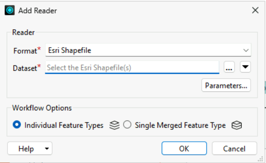
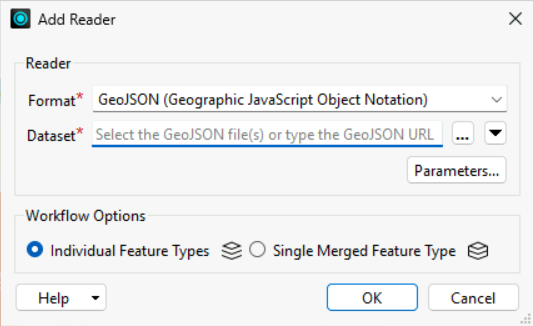
- Add the polygon and point datasets as Readers.
Add a GeoJSON Reader for the polygon dataset and an Esri Shapefile Reader for the point dataset. For each Reader, select the appropriate source file.
- Align the coordinate reference systems.
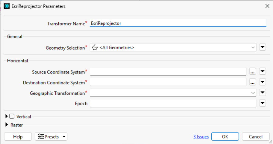
Add an Esri Reprojector to the dataset requiring transformation. Set the source CRS to that of the incoming data, set the target CRS to that of the other layer, and set geographic transformation to none. Resolve the coordinate reference system disparity between the data to be compared spatially.
- Validate the input geometry.
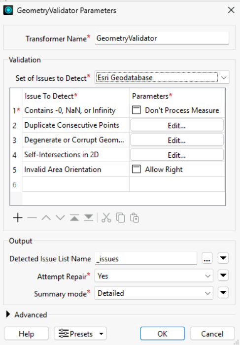
Append the polygon features to a GeometryValidator. Set the “Set of Issues to Detect” option to Esri Geodatabase. Configure the GeometryValidator to validate the presence of invalid geometry, such as self-intersection. If applicable to the data, set the Attempt Repair option, which will allow the Validator to correct invalid geometry(i.e., set the Attempt Repair option to No for point geometry).
- Perform the point-in-polygon operation.
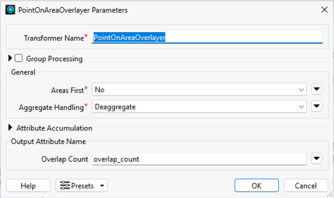
Connect the point and polygon features to a PointOnAreaOverlayer. This component validates point locations within polygon areas, transfers relevant features, and generates an overlap indicator showing how many points correspond to each polygon.
- Separate matched and unmatched points.
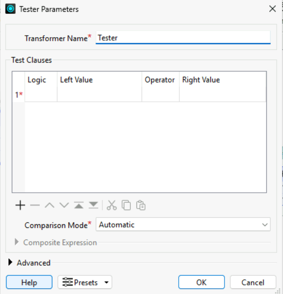
Send the point output from the PointOnAreaOverlayer to a Tester. Configure the Tester to utilize the output of the PointOnAreaOverlayer to divide the set of points that are associated with a polygon from those that are not. This ensures unmatched points are not discarded, allowing other analyses of these points.
- Set up polygon output attributes.
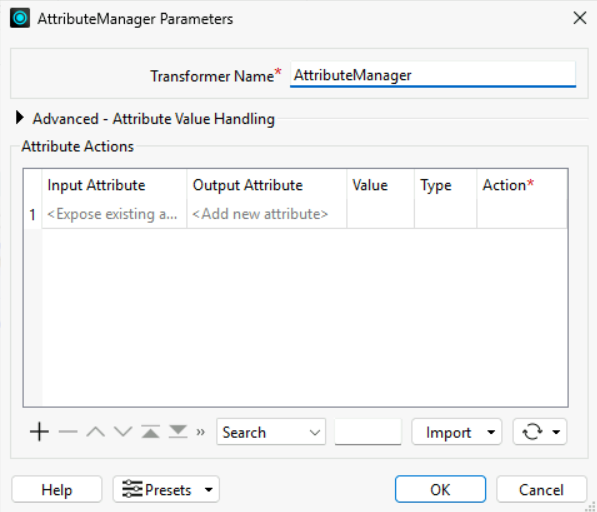
Connect the area output to an AttributeManager. Retain the polygon ID, polygon name, count of the points, and any other relevant fields for the output dataset. Delete or rename the remaining fields.
- Prepare and write the final GeoJSON output.
For web mapping, the completed polygon summary should be in EPSG:4326. Revisit step 2 for Esri Reprojection before you set up a GeoJSON Writer, specify the folder location and the final polygon output.
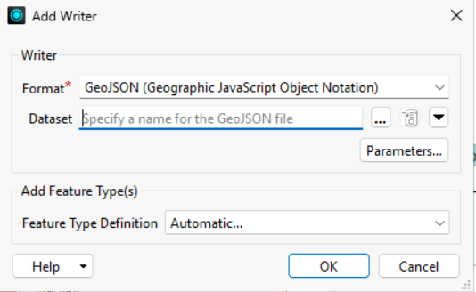
The completed workspace also brings together the same major operations as in the previous section: reading the datasets, harmonizing their coordinate reference systems, validating geometries, analyzing point-to-polygon relationships, isolating points, and creating a summary of polygons as GeoJSON.
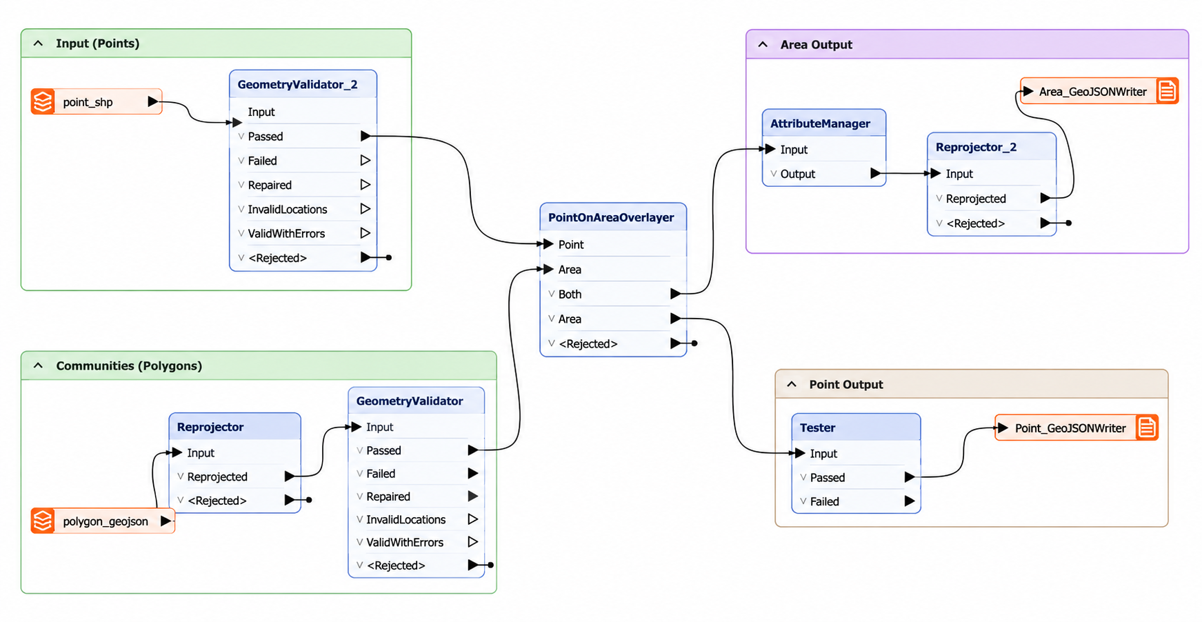
The two implementations are different. geopandas.sjoin() and PointOnAreaOverlayer are two distinct functions that handle boundaries, tolerances, and output attributes differently. When examining edge cases, you should not expect the two functions to produce the same results. However, both implementations perform the same business logic: read the polygons and points, check the CRS, validate the geometry, evaluate point-in-polygon relationships (including unmatched and multiple matches), count the points, and then save the output.
GeoPandas is an efficient library for processing vector data, especially when data volumes are not excessive. Efficiency depends on both geometry and data attribute complexity. Operations in GeoPandas are faster when you filter to only the columns and rows of interest and use more efficient reprojections. Data partitioning and/or PostGIS server-side filtering may be required when data exceeds available memory.
Recommendations
Here are some recommendations for success.
Inspect metadata before spatial operations.
Before writing any output, verify the column names, CRS, geometry types, and layer bounds. Each of these may produce output instead of an error, and output that appears correct is the hardest to troubleshoot later.
Align CRSs before comparing layers.
Set the CRS for all layers before spatial operations. Use set_crs() only for layers with unreferenced vertices to assign a CRS. Use to_crs() for layers that need to be transformed to the same CRS. Spatial operations will yield the expected results only when layers are referenced and aligned.
Validate relationships after joining.
Valid geometry and predicates do not guarantee correct results; overlapping polygons or boundary points can still produce unintended matches. To avoid this, check whether the relationships are accurate, verify how many points were matched, and confirm whether any were matched more than once.
Choose predicates from the business rule.
When working with predicates, choose the one that best fits the analysis. Avoid the selection of a predicate based simply on the quantity of results derived. This will avoid capturing technically valid results that are invalid from an analysis standpoint.
Preserve unmatched records and duplicate matches.
Use a left spatial join and retain unmatched and multiply matched records until you have investigated them. An unmatched point may lie outside the study area, fall on a boundary, or indicate a CRS or coverage problem. Removing these records too early eliminates the evidence needed to diagnose incorrect joins.
Reconcile and reopen outputs.
Compare the number of input points, matched rows, unmatched points, duplicate matches, and aggregated counts before publishing the result. After writing the output, reopen it with GeoPandas and verify its CRS, feature count, geometry types, required fields, and total counts. This validates the file downstream users will receive, not just the in-memory GeoDataFrame.
Last thoughts
GeoPandas addresses various data-handling and processing problems to improve overall functionality. These include data reliability when a CRS is missing or geometry is invalid. GeoPandas ensures that data issues are addressed during data science pipelines, automating analysis and ensuring data integrity and usability.
The article’s workflow includes loading, validating, aligning, joining, aggregating, and exporting, which is a typical spatial analysis workflow. Both GeoPandas and FME Workbench can perform these tasks; however, they use different methods.
FME Form is an integration tool that outperforms Python in scalability and operational monitoring. It includes a geometry validation transformer and a built-in cache. The choice between Python and FME Form depends primarily on budget and team skill. Still, FME’s performance and reliability make it well-suited for large data pipelines used in enterprise geospatial data governance.
Continue reading this series
Spatial Computing
Learn the basics of spatial computing and its benefits, key applications, and practical examples for processing spatial data using low-code frameworks like FME and traditional GIS software.
KML To GeoJSON
Learn about converting KML to GeoJSON files, including methods, best practices, and key differences between the two spatial file formats.
Geospatial Data Integration: Best Practices
Learn about the importance of seamless integration of diverse geospatial data sources and the challenges, best practices, and workflows involved in achieving accurate mapping and analyses for decision-making.
Shapefile To GeoJSON: Best Practices
Learn three proven methods to convert shapefiles to GeoJSON for modern web mapping applications.
Digital Twin Examples
Learn how digital twin examples are reshaping manufacturing, cities, hospitals, and farms with real-time data.
Augmented Reality Databases
Learn the key database types, data requirements, and best practices for building production-ready augmented reality systems.
MCP Server Geospatial: Tutorial & Implementation
Learn how a geospatial MCP server connects AI agents to spatial tools reliably and at scale.
Spatial Data
Learn how spatial data models, formats, and no-code automation tools simplify complex integration workflows.
What is Geospatial Data
Learn geospatial data fundamentals, real-world use cases, pipeline implementation steps, and best practices using FME.
Digital Twins in Manufacturing
Learn what digital twins are, their manufacturing use cases, and how to tackle data integration challenges while digital twins effectively.
Digital Twins in Urban Planning
Learn how digital twins in urban planning enable real-time monitoring, scenario simulation, and smarter infrastructure decisions.
GeoPandas
Learn how GeoPandas loads, validates, and joins vector data in a complete point-in-polygon workflow.
Geographic Data
Learn what geographic data is, how it works, and best practices for managing spatial data workflows.
Visual Spatial Intelligence
Learn how production systems combine spatial data and geometry to answer real-world measurement questions reliably today.