Spatial Data

Spatial data is not just about maps, coordinates, and the Earth. It can represent road networks, factory floor plans, scanned engine parts, the surface of an eyeball, or any environment where position, shape, size, and spatial relationships matter.

For years, spatial workflows depended on repetitive manual work spread across spreadsheets, GIS platforms, and custom Python scripts. Today, no-code automation tools can replace much of that complexity with visual workflows that are easier to build, inspect, test, and rerun.

This article explores spatial data models, file formats, integration challenges, and workflow best practices. It also compares a traditional Python-based conversion pipeline with a modern no-code automated workflow solving the same problem.

Summary of key spatial data concepts 

Understanding spatial data

Spatial data differs from ordinary tabular or relational data because geometry is part of its meaning, not just another attribute. A row in a table can say that a bus stop exists; a spatial feature tells you where it is, which coordinate system it uses, and how it relates to roads, parcels, or service areas.

For this reason, when working with spatial data, you have to account for both the data model and the data type. The model defines how space is represented, while the data type or format defines how that representation is stored, exchanged, and processed.

Depending on the spatial data models and formats you choose, you may encounter challenges with coordinate systems, topology, geometric precision, interoperability, file size, performance, and compatibility across tools. Many spatial workflows fail not because the data is missing but because systems interpret the same spatial

Spatial data models

Common spatial data models include:

• Vector data: Represents discrete features as points, lines, and polygons, such as addresses, routes, and administrative boundaries.
• Raster data: Represents space as a grid of cells or pixels; commonly used for imagery, elevation, temperature, and land-cover data.
• Point clouds: Represent objects or environments as dense collections of 3D coordinates, often captured by LiDAR or scanning workflows.
• 2D data: Represents features on a flat plane, such as maps, parcels, roads, and floor plans.
• 3D data: Adds height, depth, or volume — for example, to buildings, terrain, indoor environments, or scanned objects like industrial parts or anatomical structures. 
• Multidimensional data: Extends spatial data with time, spectral bands, depth layers, or other measured attributes.

Spatial data types

Common spatial data types and formats include:

• GeoJSON: Web-friendly vector format for points, lines, and polygons.
• GeoTIFF: Raster format for georeferenced imagery, elevation models, and gridded data.
• Shapefile: An older but still common GIS vector format used for data exchange.
• GeoParquet: A columnar spatial data format designed for large-scale analytics and cloud-native storage systems, including data warehouses and data lakes. One example of a dataset distributed in GeoParquet is Overture Places, which provides point-of-interest data in this format. 
• KML: A visualization-focused format commonly associated with Google Earth, Google Maps, and similar tools. It is now used mainly for visualization rather than for analytical workflows.

These formats are optimized for different use cases, from lightweight web mapping to large-scale analytics and high-resolution imagery. However, that flexibility also introduces complexity. As spatial data moves between tools, databases, APIs, and workflows, differences in projections, geometry handling, metadata support, and file structures can create significant challenges for integration and processing.

Challenges in working with spatial data

Spatial data problems rarely come from one bad file. They usually come from many “almost compatible” datasets that describe the same world in different ways. Here are some of the key concerns:

• Format fragmentation: A single workflow may need to combine GeoJSON from an API, Shapefiles from a GIS team, GeoTIFFs from an imagery pipeline, and tabular coordinates from a spreadsheet. Reading those files is only the start; the harder part is turning them into one reliable structure.
• Complexities in defining Integration rules: A reliable workflow has to normalize schemas, reproject datasets into a common coordinate reference system, standardize units, reconcile geometry types, handle resolution differences, and coerce field types before the data can be merged safely.
• Feature identity needs explicit rules: Spatial integration depends on stable identifiers, especially when the output will feed a database or recurring update process. Source IDs may be missing, reused, changed between updates, or unique only within one provider’s system, so database-backed workflows need clear primary key, foreign key, and matching rules to keep records traceable and consistent.
• Temporal and geocoding differences can make valid data misleading: Two sources may describe the same feature from different collection dates, update cycles, or validity periods. Geocoding can also resolve the same address to different locations, such as a building entrance, parcel centroid, street segment, postcode center, or approximate point, so these differences should be checked before the data is merged or published.
• Data quality adds another layer of risk: Duplicate features, missing CRS metadata, invalid geometries, topology gaps, inconsistent units, conflicting attributes, and outdated records can all produce outputs that look correct but fail in analysis, routing, reporting, or publication.
• Manual work makes risks harder to control: Repeated exports, spreadsheet cleanup, GIS clicks, and one-off scripts may solve the problem once, but they are difficult to audit, rerun, or hand off. As datasets grow or update cycles become more frequent, these informal workflows turn into operational debt.
• Technical expertise is also a constraint: Spatial pipelines often require programming, GIS knowledge, data modeling, and domain context. Python gives teams control, but it also locks transformation logic inside code. Visual workflow tools make that logic easier to inspect, adjust, and maintain across technical and non-technical users.
• Spatial data often lives in silos: GIS platforms, databases, field apps, cloud storage, APIs, and legacy file shares may each hold different versions of the same features. The goal of a strong spatial workflow is to connect those sources, standardize them early, validate the output, and make the process repeatable.

Working with spatial data: Old ways vs. new

Spatial data workflows have traditionally been built from a mix of manual GIS operations, spreadsheet cleanup, file exports, and Python scripts. That approach can work, but it often relies on a small number of technical users who understand the code, data assumptions, and failure points. Points of interest (POIs) are map-based location records that identify meaningful places and enrich them with descriptive attributes, such as name, category, address, opening hours, contact details, ratings, accessibility information, and other context relevant to search, navigation, analytics, or decision-making. In this section, we’ll use a simple POI normalization example to compare that approach with a modern automated workflow.

The task is to combine an Overpass JSON file and an Overture Places GeoJSON file into one normalized GeoJSON output. Both inputs describe points of interest, but they use different schemas, identifiers, category fields, and coordinate structures. The target output uses consistent fields, including name, source_id, poi_category, source, and point geometry.

We’ll compare two ways to build the same workflow:

• A Python workflow, where the conversion logic is written directly in code.
• A visual no-code workflow, where the same logic is built visually with readers, transformers, and a writer.

The point of the comparison is practical: Visual no-code workflows reduce the need for specialized scripting skills, making the pipeline easier for non-technical or less-technical people to inspect. 

Before diving into the comparison, for this example, you may want to obtain POI data from several online sources. This example uses data from OpenStreetMap’s Overpass API as well as data from Overture Maps Explorer.

The old way: a Python-based conversion workflow

To follow this tutorial, you’ll have to be familiar with basic Python functions, JSON handling, and the command line tools.

The Python script starts by importing only what it needs: argument parsing, JSON handling, and path management. It also defines default input and output paths relative to the script’s location, as well as the Overpass tag fields that can be used as POI categories.

#!/usr/bin/env python3
import argparse
import json
from pathlib import Path

SCRIPT_DIR = Path(__file__).resolve().parent
DEFAULT_OVERTURE_FILE = SCRIPT_DIR / ".." / "input" / "overture-pois.geojson"
DEFAULT_OVERPASS_FILE = SCRIPT_DIR / ".." / "input" / "overpass-pois.json"
DEFAULT_OUTPUT_FILE = SCRIPT_DIR / ".." / "output" / "normalized_pois.geojson"

CATEGORY_KEYS = ("amenity", "shop", "tourism", "healthcare", "leisure", "office")

#!/usr/bin/env python3
import argparse
import json
from pathlib import Path

SCRIPT_DIR = Path(__file__).resolve().parent
DEFAULT_OVERTURE_FILE = SCRIPT_DIR / ".." / "input" / "overture-pois.geojson"
DEFAULT_OVERPASS_FILE = SCRIPT_DIR / ".." / "input" / "overpass-pois.json"
DEFAULT_OUTPUT_FILE = SCRIPT_DIR / ".." / "output" / "normalized_pois.geojson"

CATEGORY_KEYS = ("amenity", "shop", "tourism", "healthcare", "leisure", "office")

In the next part of the script, the first set of helper functions keeps the main workflow readable. load_json() reads a source file, point() creates a GeoJSON point feature, and overpass_category() chooses the first available category from common OSM tags such as “amenity,” “shop,” or “tourism.”

def load_json(path):
    with path.open("r", encoding="utf-8") as file:
        return json.load(file)

def point(lon, lat, properties):
    return {
        "type": "Feature",
        "geometry": {"type": "Point", "coordinates": [float(lon), float(lat)]},
        "properties": properties,
    }

def overpass_category(tags):
    for key in CATEGORY_KEYS:
        if tags.get(key) not in (None, "", [], {}):
            return tags[key]
    return None

def load_json(path):
    with path.open("r", encoding="utf-8") as file:
        return json.load(file)

def point(lon, lat, properties):
    return {
        "type": "Feature",
        "geometry": {"type": "Point", "coordinates": [float(lon), float(lat)]},
        "properties": properties,
    }

def overpass_category(tags):
    for key in CATEGORY_KEYS:
        if tags.get(key) not in (None, "", [], {}):
            return tags[key]
    return None

Next, parse_args() makes the script reusable without changing the code. By default, it reads from the project’s input folder and writes to the output, but the user can override the Overture file, Overpass file, or output path from the command line.

def parse_args():
    parser = argparse.ArgumentParser(
        description="Normalize Overture + Overpass POIs to match the FME normalized_POIs output."
    )
    parser.add_argument("--overture", type=Path, default=DEFAULT_OVERTURE_FILE)
    parser.add_argument("--overpass", type=Path, default=DEFAULT_OVERPASS_FILE)
    parser.add_argument("--output", type=Path, default=DEFAULT_OUTPUT_FILE)
    return parser.parse_args()

def parse_args():
    parser = argparse.ArgumentParser(
        description="Normalize Overture + Overpass POIs to match the FME normalized_POIs output."
    )
    parser.add_argument("--overture", type=Path, default=DEFAULT_OVERTURE_FILE)
    parser.add_argument("--overpass", type=Path, default=DEFAULT_OVERPASS_FILE)
    parser.add_argument("--output", type=Path, default=DEFAULT_OUTPUT_FILE)
    return parser.parse_args()

Next, let’s look at the main() function, which uses the previous Python functions to do the heavy lifting: conversion and integration. The main function first processes the Overpass file. It loads the JSON, loops through each element, extracts the name, source ID, category, and coordinates, then passes the result into point() to create a normalized GeoJSON feature. The second half of main() processes the Overture GeoJSON file. It reads each feature’s properties and geometry, and extracts names.primary, categories.primary, and the Overture ID, then writes the same normalized fields used for the Overpass records.

The final block creates the output folder, writes all normalized features into a single normalized_POIs GeoJSON FeatureCollection, and prints a short summary. This confirms how many features came from each source and where the output file was written.

def main():
    args = parse_args()
    features = []
    overpass = load_json(args.overpass)

    for element in overpass["elements"]:
        tags = element.get("tags", {})
        category = overpass_category(tags)
        props = {}
        if tags.get("name") is not None:
            props["name"] = str(tags["name"])
        props["source_id"] = f'{element["type"]}/{element["id"]}'
        if category is not None:
            props["poi_category"] = str(category)
        props["source"] = "overpass"
        features.append(point(element["lon"], element["lat"], props))

    overpass_count = len(features)
    overture = load_json(args.overture)

    for item in overture["features"]:
        source_props = item["properties"]
        lon, lat = item["geometry"]["coordinates"]
        name = source_props.get("names", {}).get("primary") or source_props.get("name")
        category = source_props.get("categories", {}).get("primary")
        props = {}
        if name is not None:
            props["name"] = str(name)
        if source_props.get("id") is not None:
            props["source_id"] = str(source_props["id"])
        if category is not None:
            props["poi_category"] = str(category)
        props["source"] = "overture"
        props["lon"] = float(lon)
        props["lat"] = float(lat)
        features.append(point(lon, lat, props))

    args.output.parent.mkdir(parents=True, exist_ok=True)
    with args.output.open("w", encoding="utf-8") as file:
        json.dump(
            {"type": "FeatureCollection", "name": "normalized_POIs", "features": features},
            file,
            ensure_ascii=False,
            indent=2,
        )

    overture_count = len(features) - overpass_count
    print("Normalization complete")
    print(f"Overture normalized: {overture_count}")
    print(f"Overpass normalized: {overpass_count}")
    print(f"Total output:        {len(features)}")
    print(f"Output file:         {args.output}")

if __name__ == "__main__":
    main()

def main():
    args = parse_args()
    features = []
    overpass = load_json(args.overpass)

    for element in overpass["elements"]:
        tags = element.get("tags", {})
        category = overpass_category(tags)
        props = {}
        if tags.get("name") is not None:
            props["name"] = str(tags["name"])
        props["source_id"] = f'{element["type"]}/{element["id"]}'
        if category is not None:
            props["poi_category"] = str(category)
        props["source"] = "overpass"
        features.append(point(element["lon"], element["lat"], props))

    overpass_count = len(features)
    overture = load_json(args.overture)

    for item in overture["features"]:
        source_props = item["properties"]
        lon, lat = item["geometry"]["coordinates"]
        name = source_props.get("names", {}).get("primary") or source_props.get("name")
        category = source_props.get("categories", {}).get("primary")
        props = {}
        if name is not None:
            props["name"] = str(name)
        if source_props.get("id") is not None:
            props["source_id"] = str(source_props["id"])
        if category is not None:
            props["poi_category"] = str(category)
        props["source"] = "overture"
        props["lon"] = float(lon)
        props["lat"] = float(lat)
        features.append(point(lon, lat, props))

    args.output.parent.mkdir(parents=True, exist_ok=True)
    with args.output.open("w", encoding="utf-8") as file:
        json.dump(
            {"type": "FeatureCollection", "name": "normalized_POIs", "features": features},
            file,
            ensure_ascii=False,
            indent=2,
        )

    overture_count = len(features) - overpass_count
    print("Normalization complete")
    print(f"Overture normalized: {overture_count}")
    print(f"Overpass normalized: {overpass_count}")
    print(f"Total output:        {len(features)}")
    print(f"Output file:         {args.output}")

if __name__ == "__main__":
    main()

If you put the three parts of the code that we shared with you in one Python file and provide two POI files from the two sources we mentioned, you should get a GeoJSON file as output with the POIs from the two sources based on the new schema that includes: 

• name: The POI name, when available from the source data
• source_id: The original feature ID, preserved so the record can be traced back to its source
• poi_category: The POI category, taken from the source-specific category field or tag
• source: The dataset the feature came from, such as “overpass” or “overture”
• lon: The longitude value, included where required by the output schema
• lat: The latitude value, included where required by the output schema

The main limitation of the Python code approach is that every transformation rule is embedded in the script, so schema changes, new fields, or validation rules require technical edits and retesting. This also creates a long-term maintenance responsibility. Even when the logic does not change, the team must keep the Python environment stable, update dependencies as needed, and ensure that the script continues to run as Python versions and libraries evolve.

The low-code way: FME Workbench

Manual coding approaches are a solid choice, but they require interdisciplinary teams and substantial long-term effort and investment. The same spatial data normalization pipeline can be built in FME Workbench as a visual pipeline. Instead of reading the files, looping through records, and constructing GeoJSON features in Python, the workflow shows each source, transformation, and output step directly on the canvas. FME can automatically infer JSON and GeoJSON schemas and visually expose field mappings, so no parsing or feature-construction code is required.

The figure below shows the FME Workbench canvas for the POI normalization task.

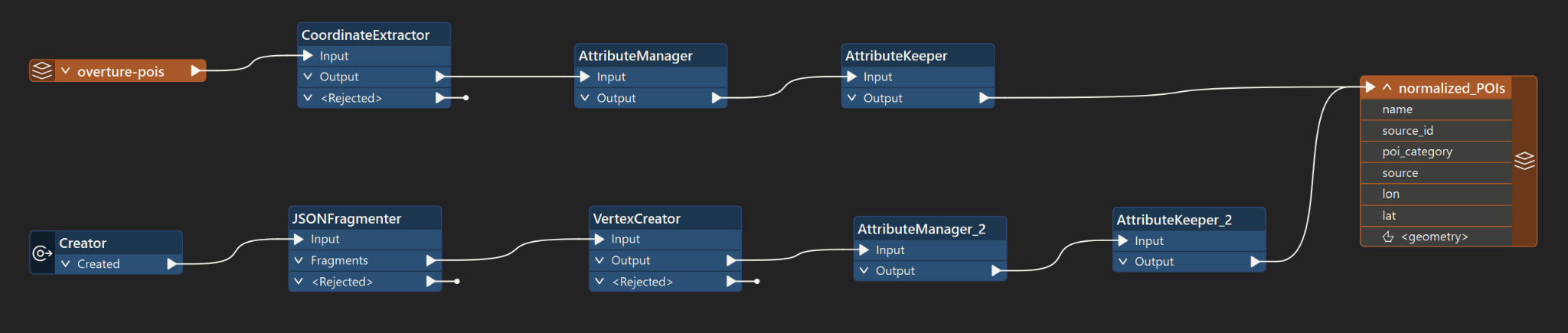
The top branch starts with the overture-pois GeoJSON file, while the lower branch prepares the Overpass JSON input through Creator and JSONFragmenter. This makes the first difference clear: Each source can keep its own structure at the start of the workflow. Overture already enters as spatial data, while the raw JSON source first has to be split into usable records.

Let’s now see how Overture data is handled. In the Overture branch (Figure 2), CoordinateExtractor writes the point coordinates into lon and lat attributes so they match the target schema. AttributeManager then renames or creates the target fields, and AttributeKeeper keeps only the fields needed in the final output.

In the Overpass branch (Figure 3):

• JSONFragmenter splits the raw JSON into usable records
• VertexCreator creates point geometry and coordinate attributes
• AttributeManager_2 maps the fields to the same target schema
• AttributeKeeper_2 retains only the final output fields

This is the visual equivalent of the Python logic that builds point geometry, assigns name, source_id, poi_category, and source, and removes unnecessary fields.

At this point, both branches feed the normalized_POIs writer (see earlier figure) with the same target fields: name, source_id, poi_category, source, lon, lat, and point geometry. This is the main advantage of the new approach. The workflow is easier to inspect, rerun, and maintain because the transformation logic is visible. A less technical user can follow the pipeline, check each transformer, and adjust the workflow without editing Python code or maintaining a Python environment.

Recommendations and best practices

Design the pipeline before you build it: Do not start by converting files one by one. First, define the source datasets, target schema, coordinate system, validation rules, expected output, and conflict-resolution logic. A clear pipeline design prevents the workflow from becoming a chain of hidden assumptions. In the FME POI example, the two-source layout makes the workflow visible from the start—one branch handles Overture GeoJSON, the other handles Overpass JSON, and both converge into the same normalized output.

Standardize early: Normalize coordinate systems, geometry types, field names, IDs, units, categories, and dimensions as close to the input stage as possible. Late standardization creates harder debugging problems because errors have already moved through the workflow. In the FME example, AttributeManager and related transformers standardize fields such as name, source_id, poi_category, source, lon, lat, and geometry for you before the records reach the writer.

Automate repeatable work: If a spatial process will run more than once, treat it as a pipeline rather than a task. Automating imports, transformations, validation checks, and exports reduces manual fixes and makes the output easier to reproduce, audit, and maintain. In the FME example, once the POI normalization workflow is built, updated Overpass or Overture files can be rerun through the same logic instead of rebuilding the process manually. If source fields change, update the affected AttributeManager mappings; the rest of the workflow can remain unchanged.

Choose formats based on the downstream use case: The best format is not always the easiest one to export. Use GeoJSON for lightweight web vector data, GeoTIFF for raster and elevation data, GeoPackage or Shapefile for GIS exchange, and GeoParquet for large-scale analytics. In the FME example, GeoJSON is a practical output format because it yields a normalized point-based POI dataset that can be reused in web mapping, APIs, or downstream spatial applications.

Validate before publishing: Add quality gates before the data leaves the pipeline. Check geometry validity, CRS metadata, required attributes, duplicate features, topology rules, units, and domain-specific constraints. In the FME example, a validation step before the normalized_POIs writer could reject records that are missing a point geometry, source_id, source, or a required category mapping.

Use the right expertise: Good spatial workflows need more than general data engineering. Engineers can design repeatable pipelines, GIS specialists can validate spatial assumptions, and domain experts can confirm whether the output makes sense in the real world. In the FME POI example, an engineer can maintain the schema logic, a GIS specialist can verify the point geometry, and a domain reviewer can confirm whether the POI categories are mapped correctly.

Use AI selectively for spatial documentation and mapping support: AI can help summarize source metadata, draft transformer documentation, or suggest candidate mappings between source categories and the target POI category field. Keep CRS handling, geometry validation, coordinate extraction, and category-mapping checks explicit in the workflow so that spatial accuracy does not depend on a probabilistic suggestion.

Track metadata and lineage: Record where the data came from, when it was processed, which transformations were applied, which checks passed or failed, and who owns the output. Without lineage, spatial data may be visually useful but difficult to trust, audit, or reuse. In the FME example, you can preserve source and source_id in the normalized output, which keeps each POI traceable back to either Overpass or Overture source files.

Conclusion

Spatial data work is rarely difficult because of a single file or format. It becomes difficult when geometry, CRS, schemas, units, metadata, and update cycles must remain consistent across systems, projects, and teams.

A Python script can be a good solution for a narrow, well-understood task. But if the workflow needs to be reviewed, rerun, modified, or handed off to someone else, a no-code visual tool approach is usually easier to maintain. The strongest spatial workflows are built for repeatability. They make assumptions visible, validate data before it moves downstream, preserve lineage, and reduce the number of manual decisions hidden inside files, scripts, or individual users’ habits.