MCP Server Geospatial: Tutorial & Implementation
Location data is everywhere: delivery apps routing drivers in real time, logistics platforms tracking thousands of assets, and urban planning tools modeling infrastructure across entire cities. What has changed is that AI agents are now expected to reason over this spatial data, not just display it.
The problem is that wiring AI agents into geographic tools has historically been messy. Engineers hardcode geocoding API calls here and routing queries there, and they end up with a patchwork of integrations that break whenever a schema changes or a new agent comes online. There is no consistency, no governance, and no way to debug when something goes wrong.
The Model Context Protocol (MCP) was developed by Anthropic to fix this problem. MCP is now an open standard, managed by the Linux Foundation’s Agentic AI Foundation, that gives AI agents a clean, structured way to call external tools. When you apply it specifically to geospatial operations and data, you get what’s called a geospatial MCP server: a purpose-built execution layer that connects AI agents to spatial capabilities safely and reliably.
This article explains what a geospatial MCP server is, how it works, and how to build one that holds up in production. We are not covering GIS fundamentals; the focus is on the architecture and the practical decisions that matter when building location-aware AI systems.
Summary of key geospatial MCP server concepts
The table below summarizes the five key concepts that this article covers in detail.
| Concept | Description |
|---|---|
| Why spatial AI integrations break | Direct GIS API calls create inconsistent, unobservable AI workflows that fail as systems scale. |
| What an MCP server does | MCP standardizes how AI agents and other applications call external tools through a governed JSON-RPC 2.0 interface. |
| Anatomy of a geospatial MCP server | A geospatial MCP server exposes spatial data, spatial operations, spatial workflows, geocoding, routing, and polygon analysis as validated, sequenced tools that the AI agent can call safely. |
| Building and governing a geospatial MCP server | Schema normalization, implementation-based token execution ordering, and OpenTelemetry instrumentation make the MCP server tools reliable in production across both spatial and broader agentic AI workflows. |
| Real-world geospatial MCP workflow | A logistics optimization agent shows exactly how MCP tools chain together to turn a natural language request into a structured spatial result. |
Why spatial AI integrations break down
Consider what happens when an AI agent needs to complete a spatial task, like resolving an address to coordinates, then calculating a route, and then checking whether that route passes through a restricted zone. Without a shared standard, the agent independently calls a geocoding API, routing API, and polygon API, and each returns data in a different schema. Each team that touches the workflow rebuilds the same capability differently. There is no shared contract and no common interface.
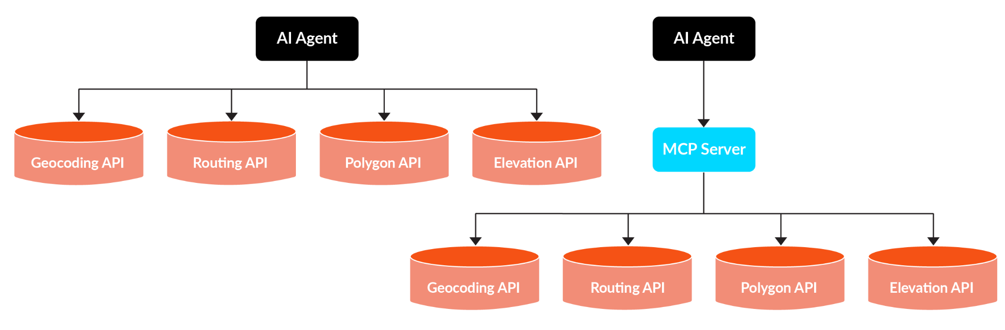
Without a shared standard, each spatial API becomes an independent integration with no consistency or traceability. To illustrate how quickly this becomes unmanageable, consider how three common geocoding services return the same data point.
| Provider | Latitude Field | Longitude Field | Address Field | CRS |
|---|---|---|---|---|
| Google Maps | geometry.location.lat | geometry.location.lng | formatted_address | WGS 84 |
| Mapbox (v5) | center[1] | center[0] | place_name | WGS 84 |
| OpenCage | geometry.lat | geometry.lng | formatted | WGS 84 |
| Legacy Municipal DB | Y_COORD | X_COORD | PROP_ADDR | NAD 83 / Local |
Three commercial providers, three different JSON paths for the same coordinate. Add a legacy municipal database returning a different CRS entirely, and the agent has no reliable way to reason over the results without custom parsing logic for each source.
The observability problem compounds the issue. With no instrumentation in this setup, platform teams cannot trace which spatial tool ran, what inputs it used, or why it failed. When a routing result comes back wrong, there is no audit trail connecting the geocoded input to the engine’s output. Errors become extremely hard to diagnose, especially when multiple agents are hitting the same spatial services with different expectations.
Enterprise spatial data makes this worse. Municipal systems and legacy databases return inconsistent field names, mixed coordinate reference systems, and colloquial location inputs that vary by region. When this unfiltered data reaches the LLM, the result is degraded reasoning and hallucinated spatial logic. For example, an agent asked to find the nearest warehouse might return a facility 100 miles away because it silently mixed up coordinate systems with no validation layer to catch the mistake.
What an MCP server does
MCP is an open standard, originally introduced by Anthropic in November 2024 and in December 2025 donated to the Agentic AI Foundation and run by Linux Foundation. (co-founded by Anthropic, Block, and OpenAI with support from Google, Microsoft, and AWS). It works as a JSON-RPC 2.0 interface that cleanly separates AI reasoning from tool execution. The agent decides what to do; the MCP server handles how it gets done.
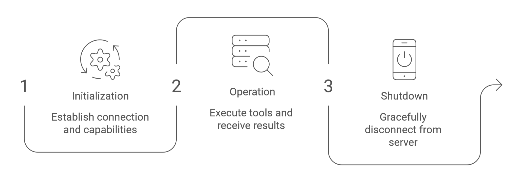
The protocol follows a three-phase connection lifecycle:
- Initialization: The server publishes its available tools so the agent (or any MCP client) can discover what it can call dynamically.
- Operation: The agent sends JSON-RPC requests to invoke those tools.
- Shutdown: The connection closes cleanly.
This lifecycle means agents never need hardcoded knowledge of what tools exist—they discover capabilities at runtime.
Here is what tool discovery looks like in practice. During the initialization step, the server responds to a tools/list request with its available capabilities:
{
  "jsonrpc": "2.0",
  "id": 1,
  "result": {
    "tools": [
      {
        "name": "reverse_geocode",
        "description": "Converts coordinates to a structured address",
        "inputSchema": {
          "type": "object",
          "properties": {
            "lat": { "type": "number", "minimum": -90, "maximum": 90 },
            "lon": { "type": "number", "minimum": -180, "maximum": 180 }
          },
          "required": ["lat", "lon"]
        }
      }
    ]
  }
}tools/list response (source)
The agent never hardcodes tool signatures. It reads this manifest at connection time and knows exactly what it can call, which parameters are required, and which constraints apply, all enforced by JSON schema before execution.
Engineers should be aware of two transport options. Stdio transport is designed for local or desktop client use where the server runs as a subprocess. Streamable HTTP is the right choice for networked production deployments where multiple agents or services need to reach the server over a network. The earlier Server-Sent Events (SSE) standalone transport is deprecated in the current specification and should not be used as a foundation for new implementations. Note that Streamable HTTP may still use SSE internally as its streaming mechanism; the deprecation applies to SSE as a standalone transport, not as a protocol primitive.
Anatomy of a geospatial MCP server
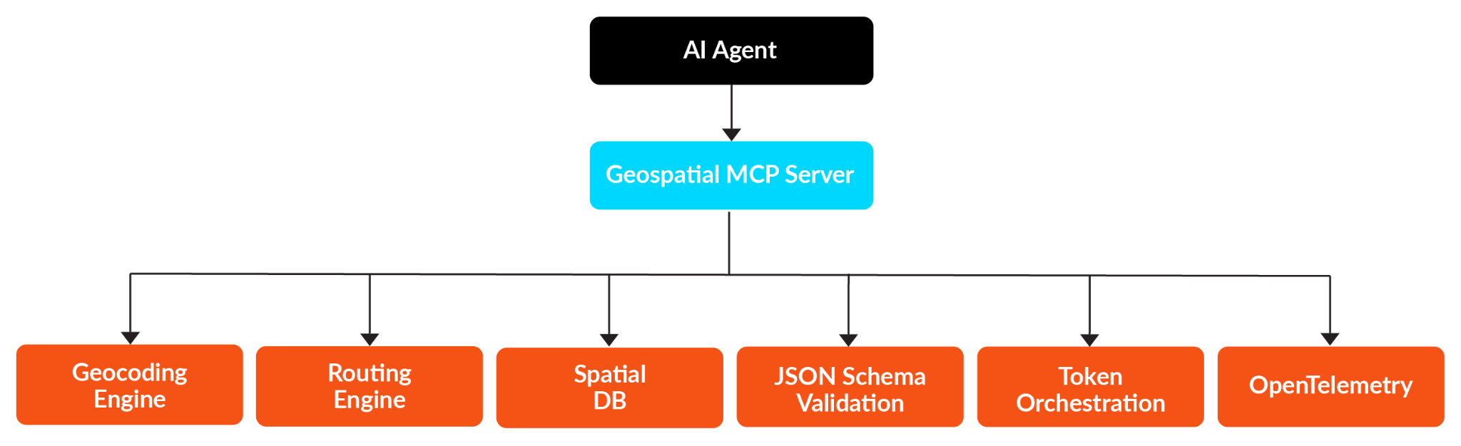
A geospatial MCP server is not a pre-built product; it is an MCP server you implement and configure specifically for spatial operations. In a nutshell, it is an MCP server capable of specialized spatial operations. Instead of the agent calling raw GIS APIs directly, it calls purpose-built tools exposed by the server, and all the underlying complexity, coordinate transformations, schema differences, and projection handling are abstracted away behind a validated interface.
The actions that a geospatial MCP server could perform typically include operations like reverse_geocode(coord) for translating coordinates to human-readable locations, find_nearby(lat, lon, radius, type) for proximity searches, route(origin, destination, constraints) for path calculation, and spatial join for containment queries. A practical rule of thumb: If implementing a capability correctly requires GIS domain knowledge, it belongs in the server, not the agent.
Here is what a geospatial tool definition looks like in practice using the Python MCP SDK.
# Defining a geospatial MCP tool with the Python SDK
from mcp.server.fastmcp import FastMCP

mcp = FastMCP("geospatial-mcp")

@mcp.tool()
async def reverse_geocode(lat: float, lon: float) -> dict:
	"""Converts coordinates to a structured address.
	Handles provider abstraction and CRS normalisation."""
	if not (-90 <= lat <= 90) or not (-180 <= lon <= 180):
    	raise ValueError(f"Invalid coordinates: {lat}, {lon}")

	# Delegate to geocoding engine (swappable)
	raw = await geocoding_engine.reverse(lat, lon)

	# Normalise response to standard schema
	return {
    	"address": raw.get("formatted_address") or raw.get("formatted"),
    	"lat": lat,
    	"lon": lon,
    	"source": geocoding_engine.provider_name
}This example shows exactly what “abstracting GIS complexity” looks like in code. The MCP server validates coordinates, delegates to whatever geocoding engine sits behind it, and returns a normalized response. The agent never sees the provider-specific JSON.
Execution Ordering
Execution order matters in spatial workflows. A routing tool cannot run until geocoding completes, and a polygon check depends on the route geometry. Token-based orchestration, an implementation pattern you build on top of MCP, resolves this issue: Each tool produces an output token that the next tool in the chain requires as input. The MCP server validates that the prerequisite token exists before executing the next step, enforcing correct sequencing without relying on the LLM to get the order right through prompt engineering alone. If the agent tries to call the routing tool without a valid geocoding token, the server rejects the request. Execution order is enforced at the server level, not through prompt engineering.
Sync vs. async execution
The choice between synchronous and asynchronous execution depends on the operation. Geocoding and proximity lookups complete in milliseconds and work well synchronously; route optimization across dozens of stops or large-scale polygon intersection analysis can take seconds or minutes and should run asynchronously. The November 2025 MCP specification introduced a Tasks primitive specifically for this kind of long-running work, where clients can issue a request, disconnect, and poll for results later. Note that the Tasks primitive is currently in an experimental stage, so verify support in your chosen SDK before building production workflows around it.
For heavy spatial processing tasks, large-scale reprojection, raster analysis, or complex network routing, platforms like FME by Safe Software are purpose-built to handle that processing as the engine layer behind the FME’s MCP server, keeping the server itself lightweight and focused on orchestration.
Upstream data normalization
Perhaps the most overlooked consideration is upstream data normalization. Raw enterprise spatial data should never reach the agent unprocessed. Building a normalization step upstream standardizing field names, reprojecting all coordinates to WGS 84, calculating bounding boxes, and validating geometry is essential. This is where most production spatial AI failures are rooted: not in the LLM or the MCP server but in inconsistent data feeding the entire chain.
Building and governing a geospatial MCP server
Here are some factors to consider in creating a server.
Observability
MCP provides no built-in observability. Engineers must instrument the stack from day one. The practical recommendation is to implement OpenTelemetry with W3C Trace Context propagation across every tool invocation. Key signals to capture include the tool name and version invoked, the full input parameters (with sensitive fields redacted), execution duration, success or failure status, and the trace ID linking the call back to the originating agent request. Without this information, debugging spatial workflows in production is guesswork.
Security and validation
A zero-trust approach to tool inputs is non-negotiable. Every tool invocation should pass through JSON Schema validation that checks types, ranges, and required fields before execution begins. If a geocoding tool expects a latitude between -90 and 90, the schema should reject, not silently pass, an input of 900. Combine this with RBAC via API tokens or OAuth 2.1 (the June 2025 MCP specification formalized servers as OAuth Resource Servers) to enforce least-privilege access. This protects against prompt injection attacks where a malicious prompt might try to call spatial tools with crafted inputs.
Audit logging
Audit logging is non-optional once the system handles sensitive location data. Each tool invocation log should capture the timestamp, authenticated caller identity, tool name, input parameters, output summary, and execution duration. For regulated industries such as logistics, defence, and urban planning, this audit trail is often a compliance requirement, not just good practice.
Real-world geospatial MCP workflow
To see how these pieces fit together, consider a realistic scenario: a logistics optimization agent that needs to plan a delivery route across 40 stops with road constraints such as bridge weight limits and time-of-day access restrictions. This scenario was chosen as a realistic, multi-step example rather than a “toy” use case. It exercises every part of the architecture discussed above, including batch geocoding, constraint retrieval from a spatial database, async execution, and token-based ordering across tools.
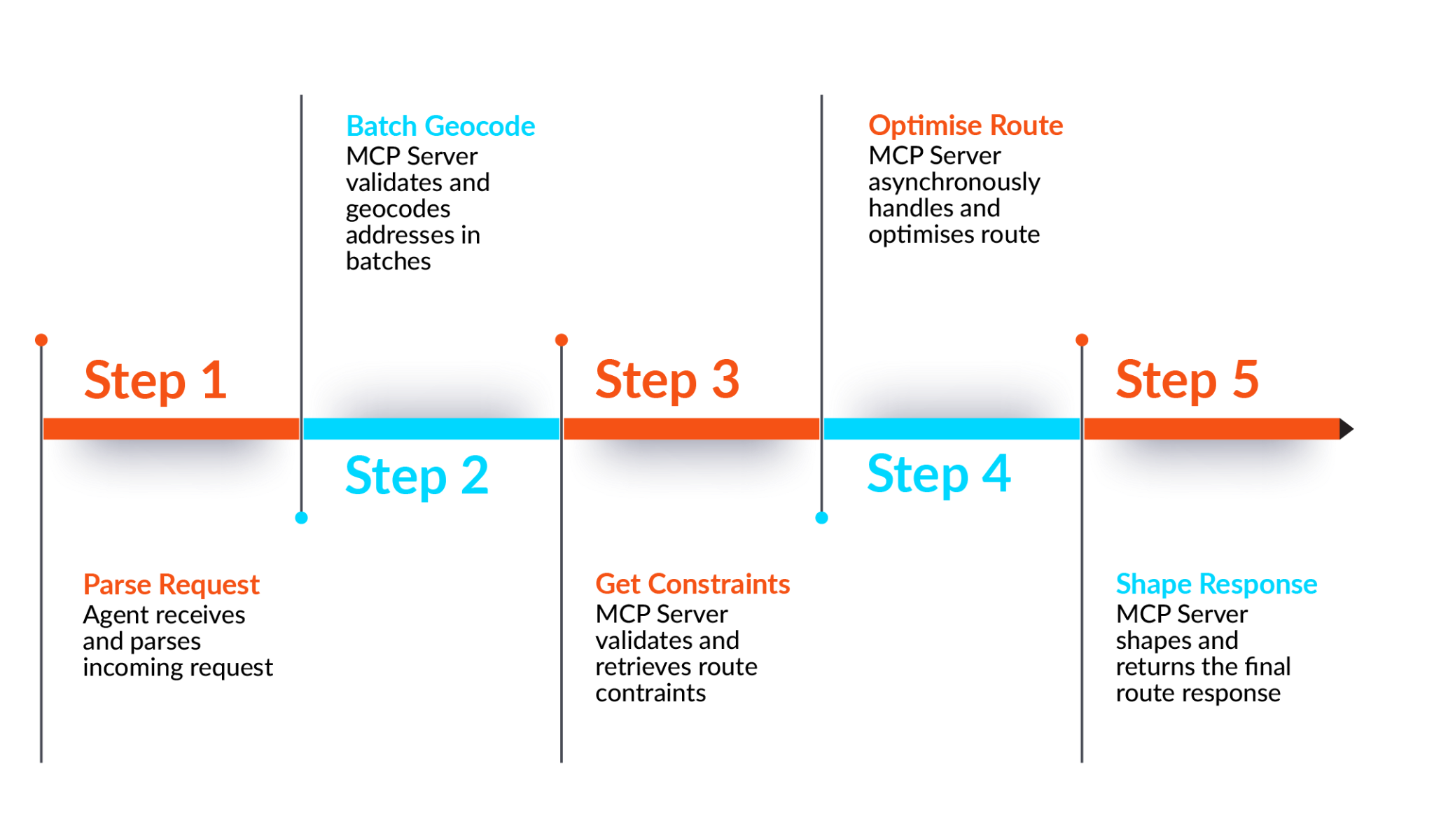
The workflow proceeds through five execution steps, each showing what the MCP server handles versus what runs in the spatial engine layer behind it.
| Step | What the agent does | What the MCP server owns | What the engine layer runs |
|---|---|---|---|
| 1. Parse Request | Extracts intent from natural language | – | – |
| 2. Batch Geocode | Calls batch_geocode | Validates addresses, normalizes input, returns token | The geocoding engine resolves coordinates |
| 3. Get Constraints | Calls get_road_constraints (gated on geocode token) | Validates token, structures constraint data | Spatial DB returns restrictions |
| 4. Optimise Route | Calls optimise_route (gated on both tokens), polls for result | Returns task handle, runs async | The routing engine computes the optimal path |
| 5. Shape Response | Presents the result to the dispatcher | Formats output to the expected schema | – |
Step 1: Natural Language Request. A dispatcher types: “Optimize tomorrow’s route for truck 14 across all 40 delivery stops, avoiding restricted bridges.” The LLM parses this into a structured intent and identifies the MCP tools needed.
Step 2: Batch Geocoding. The MCP server’s batch_geocode tool receives the 40 addresses, normalizes them, and returns validated coordinates with a completion token. The server owns the input validation and schema normalization; the geocoding engine (Google Maps, Mapbox, or an on-premise service) runs behind it.
Step 3: Constraint Retrieval. The MCP server’s get_road_constraints tool, gated on the geocoding token, queries a spatial database for bridge weight limits and time-based access restrictions along candidate corridors. The server validates and structures the constraint data; the spatial database handles the query.
Step 4: Route Optimisation. The MCP server’s optimize_route tool, gated on both the geocoding and constraint tokens, runs asynchronously. It passes the coordinates and constraints to a routing engine. The MCP server returns a task handle; the agent polls for the result. This is where clean separation matters most: the routing engine (whether OSRM, Valhalla, or a commercial solver) can be swapped without changing the agent or the MCP contract.
Step 5: Shaped Response. The MCP server formats the optimized route into the agent’s expected output schema: ordered stops, estimated arrival times, flagged constraints, and total distance. The agent receives structured, validated data and presents it to the dispatcher.
Throughout this workflow, the MCP server is the governed interface. It validates inputs, enforces execution order through tokens, delegates heavy computation to specialised engines, and structures outputs for the agent. Every step is instrumented and auditable.
Implementing the workflow with FME
The logistics workflow described above requires two capabilities that are difficult to build from scratch: a reliable spatial data normalization pipeline and a heavy async processing engine for route optimization. This is where FME by Safe Software comes in.
FME Flow now supports MCP Server capabilities directly, meaning that existing FME workflows’ reprojection, schema normalization, and format conversion can be exposed as governed MCP tools that any compatible AI agent can call securely.
In the logistics scenario, the upstream normalization step (standardizing the 40 delivery addresses, reprojecting coordinates to WGS 84, validating geometry) maps directly to an FME workflow published as an MCP tool. The route optimization step, which runs asynchronously, maps to a second FME workflow handling the heavy computation behind the MCP server’s task handle.
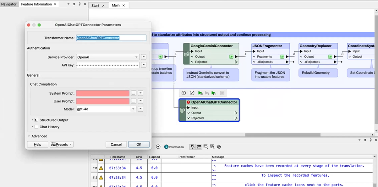
FME also includes the MCPCaller transformer, which allows FME workflows themselves to call external MCP servers, making it possible to build bidirectional integrations where FME both exposes and consumes MCP tools. For teams already running spatial data pipelines in FME, this means the path to a governed geospatial MCP server is shorter than building from scratch.
Conclusion
This article has focused specifically on applying MCP within geospatial data use cases. The architecture, tooling decisions, and governance patterns described here are designed for spatial workflows. However, many of the principles apply equally to other MCP server implementations.
A geospatial MCP server is, at its core, a simple idea: Put a governed execution layer between your AI agents and your spatial tools, and everything downstream becomes more reliable. The agent stops needing to know about GIS APIs, coordinate systems, or schema inconsistencies. It calls a tool, gets a structured result, and moves on.
What makes this worth building properly is that the reusability compounds. Once the spatial capabilities are exposed through MCP, any agent in the stack can use them without rebuilding the integration from scratch. The normalization pipeline, access controls, and observability all live in one place and serve everything that connects to them.
The upstream data layer is where this architecture either holds together or falls apart. Clean, normalized spatial data arriving at the MCP server is the difference between an agent that reasons correctly and one that hallucinates geometry. Platforms like FME are specifically built for the complex spatial data transformation and schema normalization work that makes this possible. With FME Flow now supporting MCP Server capabilities directly, organizations can turn existing spatial data workflows into governed MCP tools that agents call securely. If you are designing the spatial engine layer behind your MCP server, their data integration tools are worth evaluating at this stage.
Start with a small tool surface, wire in the observability before going live, and enforce execution order through token-based orchestration rather than prompt engineering. Getting these three things right gives you a geospatial MCP server that is built to last and built to grow.
Continue reading this series
Spatial Computing
Learn the basics of spatial computing and its benefits, key applications, and practical examples for processing spatial data using low-code frameworks like FME and traditional GIS software.
KML To GeoJSON
Learn about converting KML to GeoJSON files, including methods, best practices, and key differences between the two spatial file formats.
Geospatial Data Integration: Best Practices
Learn about the importance of seamless integration of diverse geospatial data sources and the challenges, best practices, and workflows involved in achieving accurate mapping and analyses for decision-making.
Shapefile To GeoJSON: Best Practices
Learn three proven methods to convert shapefiles to GeoJSON for modern web mapping applications.
Digital Twin Examples
Learn how digital twin examples are reshaping manufacturing, cities, hospitals, and farms with real-time data.
Augmented Reality Databases
Learn the key database types, data requirements, and best practices for building production-ready augmented reality systems.
MCP Server Geospatial: Tutorial & Implementation
Learn how a geospatial MCP server connects AI agents to spatial tools reliably and at scale.
Spatial Data
Learn how spatial data models, formats, and no-code automation tools simplify complex integration workflows.
What is Geospatial Data
Learn geospatial data fundamentals, real-world use cases, pipeline implementation steps, and best practices using FME.
Digital Twins in Manufacturing
Learn what digital twins are, their manufacturing use cases, and how to tackle data integration challenges while digital twins effectively.
Digital Twins in Urban Planning
Learn how digital twins in urban planning enable real-time monitoring, scenario simulation, and smarter infrastructure decisions.
GeoPandas
Learn how GeoPandas loads, validates, and joins vector data in a complete point-in-polygon workflow.
Geographic Data
Learn what geographic data is, how it works, and best practices for managing spatial data workflows.
Visual Spatial Intelligence
Learn how production systems combine spatial data and geometry to answer real-world measurement questions reliably today.