
Geospatial Data Integration: Best Practices
With the availability of diverse geospatial data sources today—including satellites, drones, APIs, IoT sensors, enterprise databases, BIM/CAD, etc.—seamlessly integrating these varied inputs has become extremely important for dependable analyses and accurate mapping. Integration ensures that these different datasets align in terms of semantics and location.
Integration does not mean simply overlaying the datasets. It involves the technical work of harmonizing various data types to ensure compatibility between them, so they can function within a single framework without conflict. The term “geospatial data integration” refers to the integration of location-based data from various sources, formats, and coordinate reference systems into a single framework for the analyses required for decision-making processes.
This article unpacks the central questions:
- What is geospatial data integration?
- Which data types are involved?
- What are the most common challenges?
- Are there any specific tactics or best strategies to follow?
A hands-on workflow is also presented that demonstrates geospatial data integration in both full, end-to-end code-based and no-code environments (such as Safe Software’s Feature Manipulation Engine, FME).
Summary of key geospatial data integration concepts
| Concept | Description |
|---|---|
| Differences between KML and GeoJSON | Combining geospatial datasets from various sources in one framework while guaranteeing that they align semantically and spatially with no disputes. |
| Data types and formats | Geospatial information is typically available in three primary formats—rasters, vectors, and point clouds—each with its own distinct structure and metadata. They all behave differently and require different preprocessing steps. |
| Interoperability standards | Some geospatial specifications and standards enable seamless communication among datasets, services, and applications. |
| Role of automated workflows | Automated pipelines are able to extract, transform, and load data without human error. Workflows with integrated QA/QC are made possible by both code-based or no-code platforms, but utilizing FME is a relatively better practice for smooth data integration and workflow automation because it reduces the complexity of a pipeline. |
| Challenges of integration | Spatial analyses can be disrupted by coordinate reference system (CRS) mismatches, poor georeferencing, schema drift, broken geometries, temporal misalignment, inconsistent spatial resolution, and other common challenges. |
| Best practices for geospatial data integration | • Validate and synchronize the units, metadata, and CRS of various datasets early in the workflow. • Execute the whole workflow on subsets of big data, then batch-process. • Ensure that you perform geometry fixes, mosaicking, resampling, schema standardization, etc. to prepare the data for analysis. • Enforce traceability of each step by enabling logging in the process. • Utilize no-code tools, such as FME, for smart automation. • Track variations in scripts, workspaces, or schemas in repositories. |
Understanding geospatial data integration
The handling of geospatial data requires a departure from traditional data engineering methods. Processing it is more challenging than is the case for tabular or other non-spatial data due to its geometry, geographic reference systems, topology, and varying precision levels. The way these datasets relate to one another is further influenced by variations in acquisition time and method.
Complexities are introduced by characteristics that are not found in non-spatial data. For example, LiDAR point cloud elevation information obtained in a 3D coordinate system can’t be reliably employed with 2D building boundaries (polygons) until their vertical and horizontal reference systems are reconciled.
The process of “integration” in spatial data environments involves preparing data prior to analysis to ensure that the qualities of the various datasets work together without conflicts and that they yield reliable results. It’s a technical alignment step, not merely a “visual” adjustment in GIS software, and the failure to follow this step may result in misalignment, faulty analyses, and outputs that do not accurately reflect real-world conditions.
As an example, the road system of a city collected in 2015 may not overlay properly with a 2024 satellite image of the city, as positional accuracy and feature geometry could have changed over time. Integration entails addressing issues related to temporal consistency, coordinate reference systems, and schema standardization as well as verifying and correcting geometry and ensuring overall data quality prior to analysis.
Spatial data is more useful and valuable to larger organizational systems when properly integrated. For example, databases can be linked by engineers to network infrastructure, analysts can integrate sensor observations with environmental levels, and operational teams can utilize consistent spatial information in planning programs, risk mapping models, and other applications. When datasets are standardized to a common spatial framework, they become interoperable components that facilitate a seamless flow of geospatial data into dashboards, fieldwork operations, digital twins, routing systems, analytics platforms, planning programs, and enterprise systems (such as ERP/CRM products). Both private organizations and national agencies make significant investments in robust spatial integration workflows due to their broad, cross-functional value.
Geospatial data types and formats
Today, geospatial workflow relies on information from multiple sources:
- Raster products from remote sensing missions include optical images, hyperspectral and multispectral layers, synthetic aperture radar (SAR) information, and thermal data.
- Digital elevation models (DEMs) are also rasters that can be used for terrain modeling, flood simulation, line-of-sight analysis, and other applications.
- Vector layers often depend on GIS repositories or databases.
- GIS repositories or databases provide vector layers, such as GeoJSON utility networks for water pipes, electricity lines, or fiber infrastructure.
- BIM/CAD environments give very detailed engineering plans.
- LiDAR studies produce 3D point clouds, and photogrammetric processing produces high-resolution orthophotos.
- Real-time spatial data is sent by IoT devices/sensor networks, and cloud-based APIs deliver dynamic/event-driven geospatial feeds.
- Augmented reality (AR) is also a new and emerging spatial data type and interaction mode that field workers can use to experience spatial layers directly in the real world with mobile devices or smart glasses. AR connects GIS data, 3D city models, BIM objects, or point cloud data to precise geolocations for the first time, linking office-based spatial analysis with on-site decision-making.
Despite their diversity, the majority of spatial datasets can be categorized into one of several well-known data types: rasters, vectors, and point clouds.
- Continuous surfaces on the ground are represented by raster datasets (gridded pixel data). Typical formats include GeoTIFF / COG, PNG, JPEG2000, JPEG, and ASCII grids. They are utilized for satellite and aerial images, elevation surfaces (such as DEMs), temperature maps, land cover maps, and geotemporal / time series environmental layers.
- Vector data includes points, lines, or polygons that identify parcels, waterways, transportation networks, administrative units, or points of interest. Vector geometry with attribute tables is stored in various types of formats, including Shapefile, GeoPackage, GeoJSON, KML, and GML.
- Point clouds typically consist of dense 3D observations with various properties, such as classes, intensity, or RGB, and tend to be in formats like LAS or LAZ files. They are mainly used for digital twins, modeling terrain, and urban 3D modeling.
Geospatial data integration is governed by the specific guidelines, spatial reference conventions, and technical constraints of each data type. However, the aim is the same across all formats: to create spatial information that is properly aligned, semantically suitable, and structurally consistent, so it can be blended, queried, or even examined in a unified pipeline.
Standards and interoperability
Interoperability is the base principle that enables geospatial platforms and services to transfer and receive data in a consistent and predictable way. The Open Geospatial Consortium (OGC) defines the principles for storing, accessing, transmitting, and displaying information across systems. Traditional OGC standards, such as the Web Map Service (WMS), offer pre-generated raster images, while the Web Feature Service (WFS) provides vector data for querying and editing and the Web Coverage Service (WCS) provides raster and coverage datasets for analytical workflows.
Traditional OGC services are based on Extensible Markup Language (XML) requests together with server implementations, which often require GIS clients to perform complex configurations for data integration. Newer OGC API standards make use of RESTful design principles and lightweight formats (e.g., standard HTTP methods and JSON). Formats like GML and GeoPackage serve as neutral containers for features, metadata, and coordinate reference systems, which are used in conjunction with these services.
The example below shows how a WFS endpoint is read directly into a GeoDataFrame and then stored in a PostGIS database.
import geopandas as gpd
from sqlalchemy import create_engine

# WFS URL (ArcGIS’ Sample World Cities data)
wfs_url = (    "https://sampleserver6.arcgisonline.com/arcgis/services/SampleWorldCities/MapServer/WFSServer?service=WFS&version=1.0.0&request=GetFeature&typeName=cities"
)

# 2. Read WFS directly into GeoDataFrame
gdf = gpd.read_file(wfs_url)

# Connect to PostGIS
engine = create_engine(    "postgresql://postgres:YOUR_PASSWORD@localhost:5432/your_database"
)

# Save the GeoDataFrame to a PostGIS table
gdf.to_postgis(
    name="sample_world_cities",
    con=engine,
    if_exists="replace",
    index=False
)

print("Data successfully saved to PostGIS")WFS forwards open, OGC-compatible data in open formats to GeoPandas and PostGIS for interpretation and ingestion, respectively. This is how interoperability and standards enable different systems to exchange geospatial data without requiring custom integration.
The OGC API suite embodies cloud-oriented, REST-driven protocols that have been steadily evolving in the sector. OGC API Features is the contemporary replacement for WFS and provides vector features as JSON over simple HTTP. Meanwhile, OGC API Tiles provides a consistent framework for distributing raster and vector tile pyramids, and OGC API Processes creates a lightweight REST interface for carrying out geoprocessing jobs on the server. OGC API Records introduces a standard model for describing and locating spatial metadata.
Tile-delivery standards play a crucial role in fast and scalable visualization. The most common web mapping frameworks still use XYZ tiling as their base approach. Cesium’s 3D Tiles format has become the standard for streaming large meshes and point cloud scenes in the 3D and digital twin domains. CityJSON and CityGML provide a semantic representation for urban 3D features. The OGC SensorThings API offers a single model for measurements, time series information, and device metadata, which allows real-time systems as well as sensor networks.
Cloud Optimized GeoTIFFs (COGs) allow fast, on-demand retrieval of raster segments via HTTP range requests. Geoparquet supplements the Parquet ecosystem with spatial capabilities for large-scale analytics, and formats like NetCDF and Zarr provide chunked, multidimensional storage for large scientific datasets. These standards form the interoperability framework for scalable, strong, and production-ready geospatial integration.
The role of automated workflows
As companies begin to utilize large amounts of spatial data from various systems, manual workflows become impractical and prone to errors. The use of automation ensures consistent retrieval intervals, eliminates human error, enables pipelines to handle large volumes of information, reduces turnaround times, and provides consistent outputs, even as new information is processed hourly or daily.
Automated extract, transform, and load (ETL) pipelines provide a structured and repeatable strategy for handling geospatial data at scale. Although ETL is a well-established concept in general data engineering, geospatial adaptation requires additional steps.
Extract
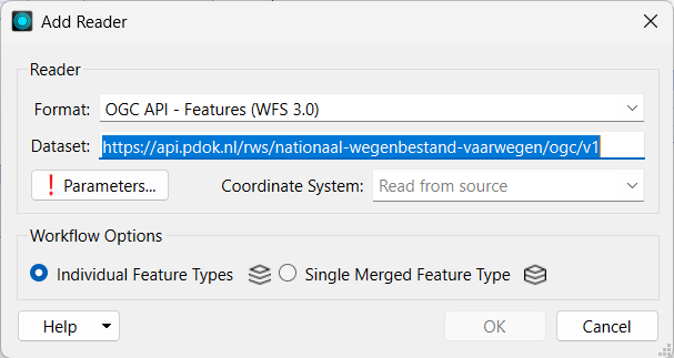
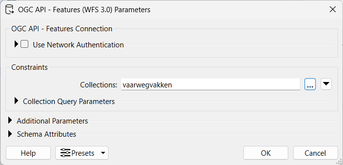
The extraction stage gathers data from different sources and presents it in a format that can be processed. Spatial extraction may involve satellite scenes downloaded from remote sensing platforms, live sensor readings via APIs, queries of enterprise geodatabases via WFS / WMS, or reading from CAD / BIM files. The Readers (see images for reference) in FME allow you to extract data from local or external sources in a simple way.
Transform
The most important step in an ETL is transformation includes several facets:
- Raster preprocessing consists of georeferencing to the correct ground coordinate system location, matching cell size resampling, mosaicking for merged imagery, and radiometric/illumination corrections for normalizing pixel values over acquisition times.
- Vector integration handles geometric validity and attribute table standardization, such as topology cleanup (filling gaps, overlaps, or self-intersections), schema alignment between datasets, and reprojection for coordinate system apposition.
- Point cloud workflows also require transformations such as classification (separating ground points from vegetation / built structures), file size limitation through thinning/decimation to minimize file size, and normalization coordination for horizontal and vertical data based on the target 3D environment.
Thus, in this step, the spatial data is validated before the main analysis. FME supplies transformers for many types of data validation and repairs (see images for some examples).
When the datasets are correctly preprocessed, they can be fed into a variety of spatial analyses, which include network routing, LULC classification, spatial joins, hazard and risk assessments, suitability modeling, and the development of specific 3D visualizations, among others.
Load
Once the data is synchronized, the loading stage transfers it to the location environment. Just as in the extraction and transformation stages, different types of data behave differently in the loading phase, necessitating distinct storage formats and methods. Depending on the workflow, outputs may be simply saved in the local machine’s drive.
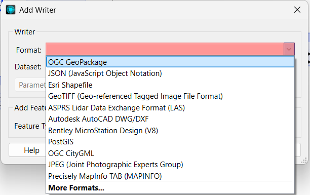
FME offers various exporting/publishing formats. Data can also be exported to formats such as GPKG/FGDB for multi-layer portable deliverables or published as web services such as WFS, WMS, or tiled layers and imported into PostGIS for big data spatial analytics, stored as Cloud object Storage in AWS S3, Google Cloud Storage, etc., in scalable access, or exported to formats such as GeoPackage / File Geodatabase. FME provides Writers (see image) that help you easily export or publish the output of your analyses in just a click.
Modern geospatial ETL pipelines can perform more than just batch processing. The same architecture is extensible for IoT sensor streams, high-velocity event data, and real-time spatial analytics. Once the ETL model has been established, it can feed data virtualization layers, drive real-time dashboards, and drive web applications that use dynamic geospatial layers.
ETL example
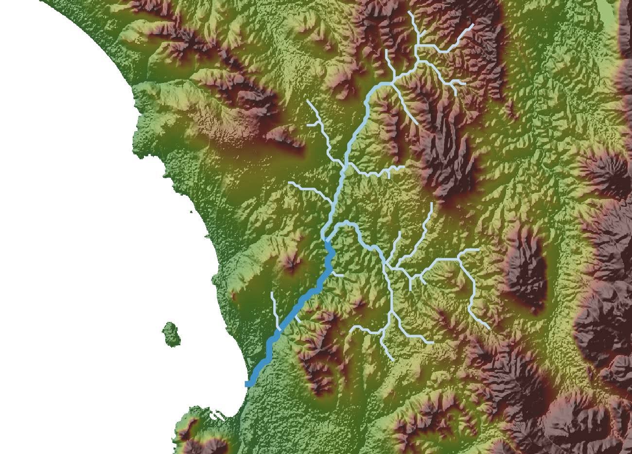
Here is a comparative analysis between code-based (Python) and no-code (FME) tools using an example of an automated workflow that extracts data from the PDOK OGC API Features service for Waterways of the Netherlands, subsets it to the Limburg province, performs geometry validation and repairs, makes 150-meter buffers around the water routes, and exports the outputs to a GeoPackage.
The code block below demonstrates how a basic ETL procedure can be implemented using Python scripting. Python provides multiple libraries, such as Requests, GeoPandas, Shapely, GDAL, etc., for this purpose.
import os
import io
import requests
from datetime import datetime, timezone
import geopandas as gpd
from shapely.ops import unary_union
import matplotlib.pyplot as plt

print("Start:", datetime.now(timezone.utc).isoformat())

# Paths and CRS
LIMBURG_PATH = "/content/drive/MyDrive/gdi/limburg.geojson"
OUTPUT_GPKG = "outputs/output.gpkg"
OUTPUT_PNG = "outputs/waterways_limburg.png"
TARGET_CRS = "EPSG:28992"  # RD New
BUFFER_METERS = 150

# PDOK OGC API for RWS waterways
OGC_API_ROOT = "https://api.pdok.nl/rws/nationaal-wegenbestand-vaarwegen/ogc/v1"

# Ensure output folder exists
os.makedirs("outputs", exist_ok=True)

# Mount Google Drive
if LIMBURG_PATH.startswith("/content/drive"):
    from google.colab import drive
    drive.mount('/content/drive', force_remount=False)
    print("Google Drive mounted.")

# Load Limburg polygon
if not os.path.exists(LIMBURG_PATH):
    raise FileNotFoundError(f"Limburg file not found at {LIMBURG_PATH}. Please upload it.")

gdf_limburg = gpd.read_file(LIMBURG_PATH)
print(f"Limburg loaded: {len(gdf_limburg)} feature(s), CRS={gdf_limburg.crs}")

# Combine into a single polygon
limb_geom = gdf_limburg.unary_union
limb_gdf = gpd.GeoDataFrame(geometry=[limb_geom], crs=gdf_limburg.crs or "EPSG:4326")

# Convert to WGS84 for bounding box (required by OGC API)
limb_wgs = limb_gdf.to_crs("EPSG:4326")
minx, miny, maxx, maxy = limb_wgs.total_bounds
bbox_wgs = f"{minx},{miny},{maxx},{maxy}"
print("Computed WGS84 bbox for Limburg:", bbox_wgs)

# Discover OGC collections
resp = requests.get(f"{OGC_API_ROOT}/collections", timeout=30)
resp.raise_for_status()
collections = resp.json().get("collections", [])
print("Available collections:", [c.get("id") for c in collections])

# Pick a collection
collection_id = None
for c in collections:
    cid = c.get("id", "").lower()
    if any(k in cid for k in ("vaar", "water", "vaarwegen", "nwb")):
        collection_id = c.get("id")
        break
if collection_id is None and collections:
    collection_id = collections[0].get("id")
print("Using collection:", collection_id)

# Fetch features
limit = 10000  # fetch up to 10k features at once
items_url = f"{OGC_API_ROOT}/collections/{collection_id}/items?bbox={bbox_wgs}&limit={limit}"
r = requests.get(items_url, timeout=60)
r.raise_for_status()

gdf_feat = gpd.read_file(io.StringIO(r.text))
print(f"Fetched {len(gdf_feat)} features, CRS={gdf_feat.crs}")

# Reproject and clip to Limburg
if gdf_feat.crs is None:
    gdf_feat = gdf_feat.set_crs("EPSG:4326", allow_override=True)

gdf_feat = gdf_feat.to_crs(TARGET_CRS)
limb_rd = limb_gdf.to_crs(TARGET_CRS)

# Keep only features that intersect Limburg
gdf_clipped = gdf_feat[gdf_feat.geometry.intersects(limb_rd.unary_union)].copy()
print(f"After clipping: {len(gdf_clipped)} features")

# Repair invalid geometries
invalid_before = (~gdf_clipped.is_valid).sum()
if invalid_before > 0:
    gdf_clipped.loc[~gdf_clipped.is_valid, "geometry"] = gdf_clipped.loc[~gdf_clipped.is_valid, "geometry"].buffer(0)
print(f"Invalid geometries fixed: {invalid_before}")

# Create buffer
gdf_buffers = gdf_clipped.copy()
gdf_buffers["geometry"] = gdf_clipped.geometry.buffer(BUFFER_METERS)
gdf_buffers.crs = TARGET_CRS
print(f"Created {BUFFER_METERS} m buffers")

# Save to GeoPackage
def save_layer(gdf, layer_name):
    if len(gdf) == 0:
        print(f"No features to save for layer '{layer_name}'")
        return
    gdf.to_file(OUTPUT_GPKG, layer=layer_name, driver="GPKG")
    print(f"Saved layer '{layer_name}' with {len(gdf)} features")

save_layer(gdf_clipped, "waterways_clipped")
save_layer(gdf_buffers, f"waterways_buffers_{BUFFER_METERS}m")

# Plot
fig, ax = plt.subplots(1, 1, figsize=(10, 10))

# Limburg boundary
limb_rd.boundary.plot(ax=ax, color="black", linewidth=1)

# Raw features (light gray)
gdf_feat.plot(ax=ax, color="lightgray", linewidth=0.4)

# Clipped waterways
gdf_clipped.plot(ax=ax, color="blue", linewidth=0.3, label="Waterway")

# Buffers
gdf_buffers.plot(ax=ax,
                 facecolor="#ff6600",
                 edgecolor="#cc3300",
                 alpha=0.35,
                 linewidth=1.2,
                 label=f"Waterway ({BUFFER_METERS} m buffer)")

# Center map
xmin, ymin, xmax, ymax = limb_rd.total_bounds
ax.set_xlim(xmin, xmax)
ax.set_ylim(ymin, ymax)
ax.set_aspect("equal", "box")
ax.set_title("Waterways in Limburg")

# Legend bottom-right outside map
ax.legend(loc="lower right", bbox_to_anchor=(1.15, -0.1), frameon=True)

# Save figure
plt.savefig(OUTPUT_PNG, bbox_inches="tight", dpi=300)
print(f"Saved map as PNG: {OUTPUT_PNG}")

plt.show()
print("Finished:", datetime.now(timezone.utc).isoformat())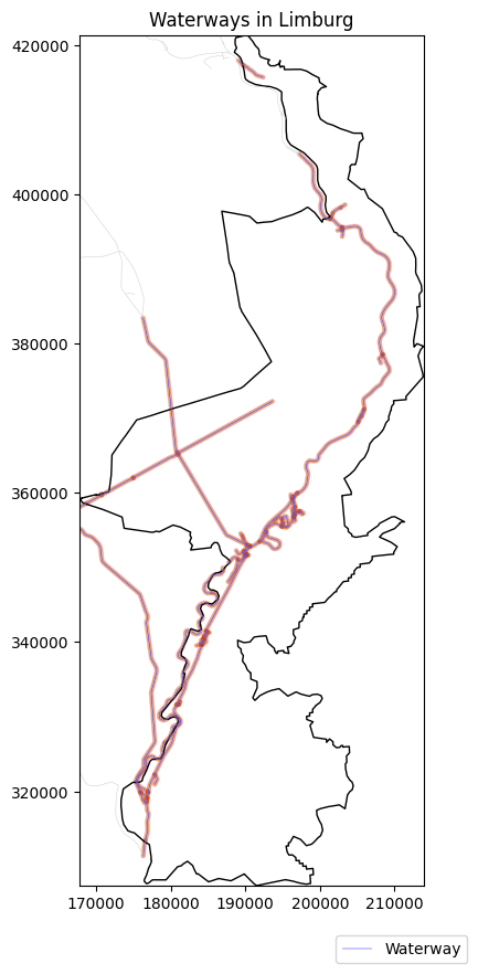
The automated workflow worked out successfully using Python. However, the script implementation required explicit management of CRS assumptions, URL construction, exception handling, geometry repair logic, file path management, logging statements’ handling, debugging, and retrying multiple times when responses were empty and malformed.
Coding-based workflows also depend on the right installation of libraries, compatible versions, and external dependencies. It can often take multiple tries to get a perfectly working script because even an extra or missing comma can open up the possibility of errors or silent failures. The outputs in Python must be plotted either through coding (non-interactively) or inspected in an external GIS software or web maps (interactively), which means that visualization must also be added to the workflow script.
On the other hand, it only took a few clicks to perform the exact same analysis in FME because it provides an interactive drag-and-drop solution to the problem.
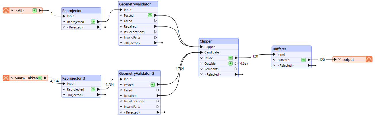
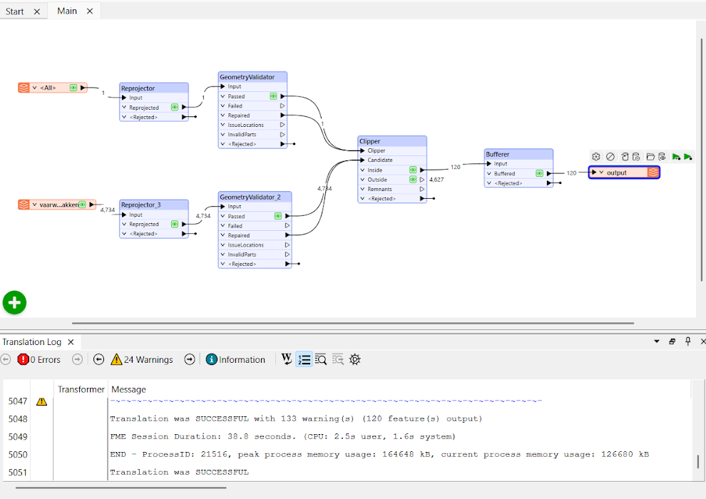
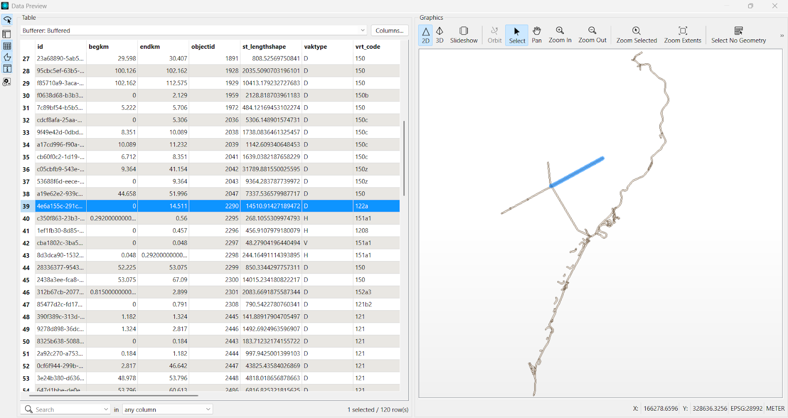
Each operation was visually encoded by readers and transformers, such as the OGC API Features reader, Reprojector, GeometryValidator, Clipper, Bufferer, and finally a writer to save in a Geopackage. Logging, verification reports, and reproducibility were built-in features within the software, saving the user from writing an additional 100 lines of code. The FME canvas also provides instant and interactive visualization of every transformation’s output. Thus, FME dramatically reduces the complexity of a workflow, making it a good choice for large datasets or scalable geospatial data automation.
Common challenges
CRS mismatch
The most common mistakes in geospatial data integration, by far. originate from CRS mismatches. Datasets often originate in different coordinate reference systems and thus misalign positional coordinates unless reprojected to a common system. Ensure spatial alignment of all datasets to a common CRS at the start of the workflow with GeoDataFrame.to_crs() in Python or FME’s Reprojector transformer.
Incorrect georeferencing
Manual georeferencing introduces uncertainty, which means that aerial imagery, scanned traditional maps, or GPS-collected observations may not match ground locations, causing apparent spatial shifts. Even a shift of a few meters can skew the analysis. Fixing this can be done by explicitly assigning or overriding the geo reference configuration in Python using set_crs() when coordinates are correct but not defined. In FME, simply apply affine shifts and ground control–based corrections using transformers like AffineWarper or RubberSheeter.
Differences in spatial resolution
Rasters with different pixel spacings cannot align perfectly. Merging low-resolution raster data with high-resolution images or LiDAR creates inconsistencies in detail, analytical accuracy, and scale. Normalize raster resolution using gdalwarp in Python or FME’s RasterResampler to avoid this issue.
Temporal inconsistencies
Data collected at different times can’t be incorporated or even used in an equivalent downstream process. Such unsynchronized data show incorrect results for change detection and other applications that rely on temporal data.
Attribute and schema mismatches
Anomalies in attribute table structure, data types, field names, and other areas hinder seamless joins and necessitate schema standardization prior to integration. Standardize attributes and schemas using pandas / GeoPandas transformations or with FME’s AttributeManager.
Topology and geometry problems
Self-intersecting polygons, duplicate geometries, overlaps, sliver polygons, and overall corrupt or invalid geometries may affect spatial analyses. Invalid geometries can be detected and repaired using Python’s buffer (0) approach or detected with FME’s GeometryValidator transformer. Other transformers can follow such as Snapper, or Intersector, etc. to attempt to repair. In many cases, identifying the geometry problem is the best that can be done.
Datums and vertical reference systems:
Elevation datasets (or maybe 3D designs created on various datums) can sometimes produce incorrect height values and also misrepresent terrain characteristics. Transform horizontal/vertical datums explicitly to avoid elevation offsets using GDAL-based transformations in Python.
Data quality
Noise coming from sensors, digitization blunders, missing attributes, or data outliers creates uncertainty in the evaluation. Use validation logic in Python (e.g., isnull(), value thresholds, drop_duplicates()), or do the same things in FME with transformers such as AttributeValidator, Tester, and DuplicateFilter.
Best practices
Validate CRS and metadata early
Ensure that all datasets have the appropriate and matching coordinate reference systems and that their metadata is consistent (resolution, acquisition time, units, etc.). One of the most important steps in any spatial analysis is to confirm the CRS of all the involved datasets and reproject them to a common system before running any analysis. This can allow you to avoid positional shifts. Early validation of metadata also prevents semantic misinterpretations that may occur further down the pipeline.
Test on a subset before scaling up
In the event of large amounts of big geodata, operate the workflow on a small test initially to identify troublesome areas. Try the workflow on the subset and adjust as necessary. Running the analysis on a small area of interest can help point out the invalid geometries, CRS mismatching issues, and other inconsistencies, which is very helpful in the long run. After the workflow is confirmed and finalized, apply it to the remaining data through batch processing.
Enforce data validation and quality control
Data preparation, or preprocessing steps such as geometry checks, topology fixes, schema normalization, unit standardization, and attribute cleaning, must be carried out before the primary analysis. One of the most important aspects is that spatial analyses rely heavily on clean geometries and accurate data. Issues such as self-intersecting lines, null values, gaps, and sliver polygons can disrupt even minor analyses, including buffering and subsetting. This is why multiple automatic and manual checks should be done before running any workflow. Analytical uncertainty is reduced by quality inputs.
Employ logging
Log every workflow execution, which includes validation outputs, errors, and all the carried out transformation steps. Logging allows fast traceability, debugging, and auditing/rollback. In Python, this is best done with either a bunch of simple print statements or a properly structured logger (with multiple lines of code).
FME logging is automatic and very easy to read in the software’s interface. Each transformer in FME reports warnings, data counts, and process failures. Good logging should be able to catch mismatches in CRS, failed API requests, or invalid geometry before they produce the wrong outputs.
Maintain version control
Store scripts, schemas, and FME workspaces in Git to track changes, ensure reproducibility, and facilitate group collaboration. Version control systems allow analysts and developers to replicate results, roll back broken changes, and document when transformations were added or modified. Version control keeps the analyst in a “safe zone,” meaning that you can make changes during a trial-and-error situation without worrying about breaking the entire workflow. It is particularly helpful for long-term geospatial projects where standards, schemas, or external APIs keep changing.
Embrace no-code automation wherever possible
Best practices for geospatial integration pipelines include automating them to ensure consistency, reproducibility, scalability, and, most importantly, to minimize human error. FME eliminates hundreds of lines of code and potential bugs by separating different phases of a workflow into different visual transformers. In our ETL example, FME did the same tasks as the Python workflow in minutes without environment setup or dependency management. Logging, debugging, schema mapping, QA checks, and reruns are also included, which make the workflow stable in production. FME dramatically reduces the complexity of a workflow, making it the best choice for geospatial data automation.
Conclusion
Geospatial data integration must be performed to obtain reliable insights from multiple source spatial datasets. With datasets growing in volume, diversity, and frequency of availability, the consistency of formats, standards, coordinate systems, and semantics determines the reliability of every downstream analysis. Strong integration methods are necessary as businesses increasingly utilize satellite images, sensor networks, or cloud-hosted geospatial data.
Automated ETL operations assure repeatable and flexible processing, and the best option for no-code/hassle-free workflows is to utilize FME. By utilizing structured integration practices, organizations can turn dispersed spatial inputs into coherent datasets that can facilitate better and more effective decisions.
Continue reading this series
Spatial Computing
Learn the basics of spatial computing and its benefits, key applications, and practical examples for processing spatial data using low-code frameworks like FME and traditional GIS software.
KML To GeoJSON
Learn about converting KML to GeoJSON files, including methods, best practices, and key differences between the two spatial file formats.
Geospatial Data Integration: Best Practices
Learn about the importance of seamless integration of diverse geospatial data sources and the challenges, best practices, and workflows involved in achieving accurate mapping and analyses for decision-making.
Shapefile To GeoJSON: Best Practices
Learn three proven methods to convert shapefiles to GeoJSON for modern web mapping applications.